Movement generation for robot arms - Kinematics and Attractor Dynamics for manipulators - Lecture 2019 (preliminary)
←
→
Page content transcription
If your browser does not render page correctly, please read the page content below
Movement generation
   for robot arms
Kinematics and Attractor Dynamics for manipulators
robotic arms
  they aren’t vehicles
movement generation for
            vehicles
•   the floor is a 2D environment

•   vehicle treated as point

•   task: reach goal

•   task: avoid obstacles

•   not much more vehicles can
    do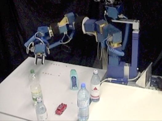
arms: what changes?
•   where we move: environment: 3D

•   what we do: more tasks are
    possible at the same time or in
    sequence: e.g. manipulation

•   an interesting point on the arm is
    the end-effector

•   what we move: chain-of-links or
    segments geometry (kinematic
    chain)

•   but moving a link can affect other
    links. complication.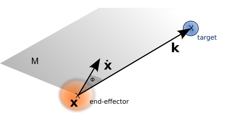
arms: what changes?
•   different tasks active at
    different times: system needs
    to combine tasks that switch
    on/off all the time

•   does Attractor Dynamics
    approach scale-up? what
    happens when multiple tasks
    are active at the same time?
    does it work? why?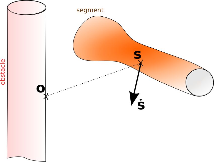
rigid bodies
•   cannot treat robot as single point
    in space, anymore

•   connected links

•   orientation and translation for
    each link: two times 3 dimensions

•   we need a way to relate our task
    to the links translation and
    orientation

•   note: not always require specific
    orientation and specific translation
    for link at the same time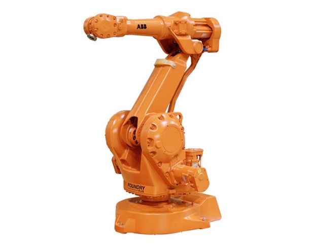
kinematics and kinetics
•   kinematics: movement
    without forces

•   kinetics: (dynamics, not in the
    mathematical sense)
    movement with forces

•   important acting forces:
    gravitation, interaction of links

•   we push kinetics out to low-
    level controller. modern robots
    know their own dynamics.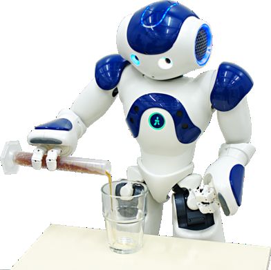
how does the arm move?

•   joints: revolute, spherical,
    cylindrical, prismatic

•   how many DoF and what kind
    of joints does the human arm
    have?

•   typically position controlled
    servo-motors
formal constraints
•   workspace: either the environment or sometimes space of reachable positions        p or x
    (vectors) of the end-effector. Euclidian.

•   configuration space: space of all possible (here:) joint positions
    space.
                                                                         ✓ (vectors). Also joint
•   task constraints: equations (equalities or inequalities) that need to be successfully
    satisfied for the task. can be vector-valued.

•   holonomic constraints: expressible purely via configuration (and time). Reduces
    dimension of workspace.

•   non-holohomic constraints: Velocity-based constraints. Introduces path-dependency.
    Typically vehicles are non-holonomic robots (can’t move side-ways).

•   Degrees of Freedom: dimensionality of configuration space.

•   Redundancy: Compare DoF and dimensions of task contraints. More DoF than
    necessary? Infinite solutions to constraints possible.
Kinematics
where is the hand?

                                                         p(✓)
•   forward kinematics

                                        l1 sin ✓1
•   example: single revolute joint
               ✓               ◆
                   l1 cos ✓1
•   p(✓1 ) =
                   l1 sin ✓1
•   generally: p is a function of   ✓                ✓
                                                    l1 cos ✓1
                                                            l1
where is the hand?
• forward kinematics
p(✓)
• example: revolute joint and
prismatic joint
p(✓) = p(✓1 , ✓2 )
✓ ◆
l2
l1 + ✓1 + l2 cos ✓2 ✓2
=
l2 sin ✓2
l1 ✓1what happens if I move a
joint?
• differential (forward)
kinematics ṗ = J ✓˙
• (kinematic) Jacobian matrix J
!
@p1 (✓) @p1 (✓)
@✓1 @✓2
J= @p2 (✓) @p2 (✓)
@✓1 @✓2
✓ ◆
1 l2 sin ✓2
=
0 l2 cos ✓2what happens if I move a
joint?
(the first joint is the prismatic ‘slider’ joint)
!
@p1 (✓) @p1 (✓)
@✓1 @✓2
J= @p2 (✓) @p2 (✓)
@✓1 @✓2
✓ ◆
1 l2 sin ✓2
=
0 l2 cos ✓2
ṗ = J ✓˙what happens if I move a
joint?
!
@p1 (✓) @p1 (✓)
@✓1 @✓2
J= @p2 (✓) @p2 (✓)
@✓1 @✓2
✓ ◆
1 l2 sin ✓2
=
0 l2 cos ✓2
ṗ = J ✓˙what happens if I move a
joint?
• differential (or instantaneous) kinematics provide a
relationship between velocities @p(✓)
ṗ = J ✓˙ J=
@✓
• note: J changes when ✓ changes
• what happens when J is singular? kinematic
singularity. rank changes
• since J changes, these singularities can appear and
disappear (at certain configurations) while moving
• nullspace of J: space of all ✓˙ that project to a ṗ of 0.how do I get the hand to
where I want it?
• we now need to look at the
inverse problem: what joints do
I need to set to what values to
reach a certain point in
workspace?
• closed form solution (inverse
of the forward kinematics)
• the forward kinematics p(✓)
can in general not be
analytically inverted
• geometrical construction.
depends on geometry of robot!how do I get the hand to
where I want it?
✓1 = arctan2 (y, x) ±
l2
✓2 = ⇡ ± ↵
✓ 2 ◆ (x, y)
1
2
l1 + l2 r 2 l1
↵ = cos ↵
2l1 l2
✓ 2 2 2
◆ r
1 r + l 1 l2
= cos
2l1 l2how do I get the hand to
where I want it?
• the differential kinematics
may be simpler to invert?
dp dp d✓
ṗ = = = J ✓˙
dt d✓ dt
• … if J is invertible.
• is J singular?
• is J even quadratic?
• iff invertible: ✓˙ = J 1
ṗ
we can calculate a commanded joint
velocity
• integrate ✓˙ to ✓ to send commandsinverse of differential
inverse of differential
kinematics
kinematics
• if J is not invertible we can use the
Moore-Penrose
• if pseudoinverse
J is not invertible, we can
. + instead
Juse of J
the Moore-Penrose
1
pseudo-inverse
• defined as:
+ +T T T 1 1 T
J =JJ =JJ
(JJ ) J
•• to invert the equation:
a generalized matrix inverse
ṗ = J ✓˙
• ✓˙ = J + ṗ
• (apply from the left) to get:
˙✓ = J + ṗ ˙
• property: minimizes |✓|
• this is a commonly used
generalized matrix inverseinverse of differential
inverse of differential
kinematics
kinematics
• J +
in ˙
✓ = J +
ṗ has useful
• ifproperties:
J is not invertible, we can
use the Moore-Penrose
• if there are many solutions
pseudo-inverse
(typically yes) it minimizes:
+ T T 1
J = J|✓|
˙ JJ
• anet
• effect: thismatrix
generalized prefers lower
inverse
speeds over all joints than one
• ✓˙ = with
joint J + ṗhigh speed. Good!
| ˙
✓|
•
• property: minimizes
if there is no solution it finds
the solution with the smallest
errorinverse of differential
inverse of differential
kinematics
kinematics
• not implemented in this manner,
• if J is not invertible, we can
though:
use the + Moore-Penrose
T 1 T
J = (JJ
pseudo-inverse
) J
• but as singular value decomposition
+ T T 1
J = J JJ T
J = U ⌃V
+ + T
• J = V ⌃matrix
a generalized U inverse
•• where
˙ U and D are specific
+
orthogonalṗmatrices and ⌃ is a
✓ = J
diag matrix of ‘singular values’ - all
• based on the
property: Eigenvalues
minimizes ˙ and
|✓|
Eigenvectors of JJ T and J T Jmore on the Moore Penrose
Pseudo-Inverse
• if ⌃ is a matrix of ‘singular values’ in the diagonal entries
• then ⌃ + is the transposed matrix of the
reciprocal values: 1
• PROBLEM: the singular values become very small when we
get close to singularities (directions in which we cannot
move)
• workaround: use the damped pseudo-inverse with the
corresponding entries: 1
+✏Attractor Dynamics for robot arms
recap: tasks in Attractor
               Dynamics
•   task as differential equation             ˙ = f( )
                                              ˙=0
•   task is adhered-to if system is
    in a fixed-point

•   move quickly into attractor
    state

•   in reality: near attractor
    suffices
                                      d /dt
•   avoidance: repellors

•   task akin “forcelet”
                                                 repellor
generating complex movements
different tasks

•   reach bottle           •   hand position, bottle position

•   grasp bottle           •   hand orientation, hand
                               opening, hand closing
•   pour the drink
                           •   bottle orientation, glass
•   put bottle on table        position, glass filling

•   avoid obstacles        •   obstacle positions, if any
different tasks
• different variables ” ”are
relevant for different tasks
• a task can be expressed as
constraint on that variable (stable
fixed-point in a dynamical system)
• but how do and ˙ relate to ✓
and ✓˙ in joints? ˙ = f( )
• task defines submanifold on =?
configuration space
• different tasks live on different
sub- manifolds of configuration
space. how can this work?independent stabilization
• independent forcelets
• each a (possibly different)
relevant variable
• constraints expressed as
attractors/repellors in
2
dynamical system over that
relevant variable only 1.5
1
• find joint space changes that
0.5
realize this task
(independently) 0
−0.5
−2 −1.5 −1 −0.5 0 0.5 1reintegration of independent
tasks
task constraint realized
• superposition of independent
forcelets
• now new vector field realizes
compromise of tasksreintegration of independent
tasks
joint angles
that realize
task 1
(hand position)reintegration of independent
tasks
joint angles
that realize
task 2
(hand orientation)reintegration of independent
tasks
joint angles
that realize
task 1
and
task 2reaching
v
k
preaching
• deviation angle dynamics,
analogously to heading angle
dynamics (define a plane M)
⇥˙ = fdir = sin ⇥
• angle: = ](ẋ, k)
• insert a step: In workspace,
what vector would realize the
change?reaching
v
k
v?reaching
v
k
v?
• from geometry we can find: ✓ ◆
⇥k, v⇤ |v|
v? = k v hk,vi
⇥v, v⇤ |k hv,vi v|
• transformation of forcelet into
workspace:
fdir = fdir · v? = sin ⇥ · v?reaching
• transformation from
workspace into joint-space: v?
• per inverse differential
kinematics:
+ T T 1
J =J JJ
+ +
Fdir = J · fdir = sin ⇥ · J · v?
• we now have a “forcelet” in
joint spacespeed
v
• analogous to the vehicle
scenario, speed treated as
independent task:
• v = |v|
• select a desired speed: vdes
fvel = vel (v vdes )
v
• v̂ =
|v| fvel = fvel · v̂
Fvel = J + · fvelobstacle avoidance
obstacle avoidance
• finding a instantaneous joint change that enacts the
required (instantaneous) task change: find direction
that moves the relevant task variable into its
attractor
• other take on it: find direction that moves the
relevant task variable away from its repellor
• problem: all links must be able to avoid. but moving
proximal links also moves distal ones (kinematic
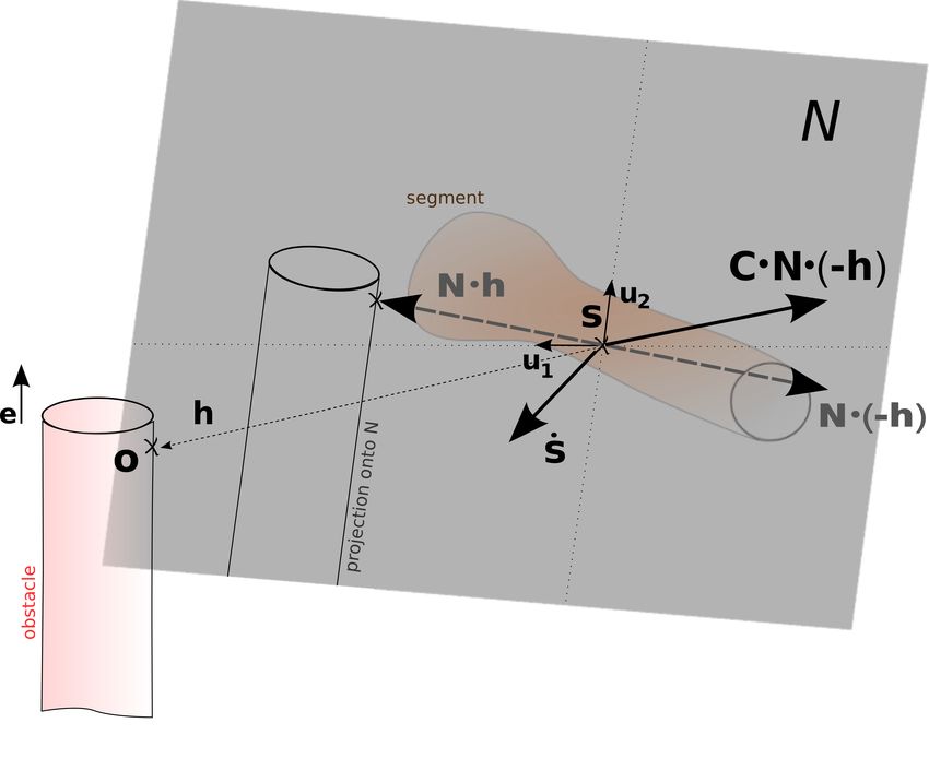
chain)for every link:
• find closest points o on obstacle and s on link
• in what direction does link point s currently move?
• in what direction should it move?
note: s does not have the same
forward kinematics and not the
same Jacobian as the end-
effector!construction on normal
plane
segment
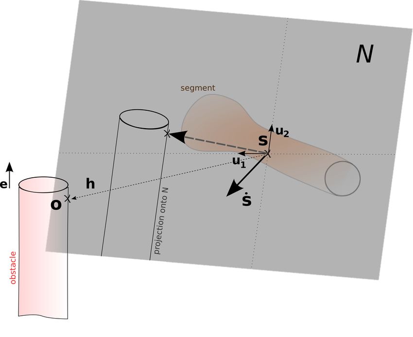
“shadow of obstacle” on plane Navoidance with upwards
bias (rotated)
segment
direct avoidanceother parameters
• distance range
• angular range
v
dgripper orientation
fori = sin ⇥
• angle dynamics
• different geometrical
construction and Jacobian
but same principle
• requires one DoF of the
system, thus preferable
only enforce when
necessary. NOT ALWAY ONsuperposition of tasks
• finally, superpose all
independently stabilizing
vector fields:
X
F = Fdir + Fvel + Fobs
obs,seg
• interpret the vector-field as
acceleration command:
✓¨ = FYou can also read