NOISE ANALYSIS OF NIKON D40 DIGITAL STILL CAMERA
←
→
Page content transcription
If your browser does not render page correctly, please read the page content below
NOISE ANALYSIS OF NIKON D40 DIGITAL STILL
                       CAMERA
                                      F. Mojžı́š, J. Švihlı́k
              Deptartment of Computing and Control Engineering, ICT Prague

                                             Abstract

      This paper is devoted to statistical analysis of Nikon D40 digital still camera.
      There are described basic kinds of image degradations like noise types and other
      distorsions. Imaging systems with their noise sources are also discussed. Main
      part is dedicated to noise analysis of imaging systems and Opto-Electronic Con-
      version Function determination.

1     Introduction

Noise in signal processing [1, 2, 6, 8] represents unwanted information added to the original
pattern (signal). There exist many kind of noise and noise sources that influence result signal.
This paper is devoted to the noise analysis of imaging systems and mentioned methods are
further applied to Nikon D40 SLR digital still camera.
Introductory part describes basic image degradations and their models, introduces term imaging
systems, focuses on their basic description, important parts like optical systems, image sensors,
etc.
Methods of imaging systems analysis used in this arcticle are largely based on international
standards ISO 14524(E):1999 and ISO 15739(E):2003, which include basic instructions deal-
ing with procedures of Opto-Electronic Conversion Function (OECF) and noise characteristics
determination, respectively.
Most of the methods desrcibed in ISO 15739 are based on simple statistical computations and
concern basic noise characteristics like standard deviation and Signal to Noise Ratio. In this
paper there is also concerned evaluation of noise dependence on changes of input signal level,
i.e. changes of noise standard deviation in OECF patches of used test chart. Except noise
analysis OECF as a relationship between input and output values of the imaging system is also
evaluated. Contrary to noise analysis that process grayscale form of the used test chart, OECF
is determined for all colour channels (R, G, B).
Probability distribution of the noise in the whole spectrum of grayscale was tested using image
histogram of the analyzed test chart. For this purpose were applied statistical distribution tests
like χ2 test of goodness of fit and Kolmogorov-Smirnov test. Generalized Laplacian Model was
used too, when mentioned statistical tests failed.

1.1   Image degradations

Images acquired by the digital cameras generally contain noise related to digitizing of the real
pattern. It means that quality of the final image is influenced by the type and quality of the
imaging system, especially by the type of image sensor used in this system. CCD and CMOS
sensors are two types of commonly used image sensors in these systems. Except sensing elements
quality, there are more sources that can influence result image, e.g., degradation due to atmo-
spheric conditions, degradation due to relative motion between the object and the camera, etc.
Degradation process [1, 8] can be described as a degradation function h(x, y) that together
with aditive or multiplicative noise n(x, y) in combination with an input image f(x, y) produce
a degrade image g(x, y).
Inverse process, when we want to obtain estimate of the original image, is called restoration.
The main purpose of image restoration is to obtain bf(x, y) function, which is an estimate of the
original image based on some knowledge, usually estimation, of the degradation function h(x, y)
and noise term n(x, y).
Image degradation model with aditive noise [1, 8] (signal independent)and model of image
degradation with multiplicative noise [1, 8] (signal dependent) are given by following relations
g(x, y) = h(x, y) ∗ f(x, y) + n(x, y) (1)
g(x, y) = h(x, y) ∗ f(x, y) · n(x, y) (2)
where ∗ is a convolution operator. Transformation between aditive and multiplicative noise
models is given by equations
eg = eh∗f+n = eh∗f · en (3)
log(g) = log(h ∗ f · n) = log(h ∗ f) + log(n) (4)
where g = g(x, y), f = f(x, y) and n = n(x, y).
Principal sources of noise in digital images arise during image acquisition and/or transmission.
Performance of imaging sensors used in imaging systems is influenced by a variety of factors.
When we expect image degradation only by the degradation function h(x, y), it means n(x, y) =
0, then result image can be expressed
g(x, y) = h(x, y) ∗ f(x, y). (5)
Main principals of estimating the degradation function are observation, experimentation and
mathematical modelling [8]. In following paragraphs there are described two mathematical
models of degradation functions. The first one is atmospheric turbulence, in the frequency
domain expressed as follows
5
2 +l2 ) 6
H(k, l) = e−c(k (6)
where c is a constant that depends on the nature of turbulence. Second model is defocusing by
the thin lens, in the frequency domain given by equation
J1 (cr)
H(k, l) = (7)
cr
√
where r = k 2 + l2 and c is a displacement. In the following paragraphs we will expect degra-
dation of the final image only by the noise, i.e., by aditive or by multiplicative
g(x, y) = f(x, y) + n(x, y) (8)
g(x, y) = f(x, y) · n(x, y). (9)
Noise in digital images can be described as a statistical quantity. It means that it is a ran-
dom variable described by its probability density function (PDF) or probability mass function
(PMF) [5]. Noise models [1, 2, 6, 8] that can be used for description of noises present in imagingsystems are Gaussian, Reyleigh, Erlang, Exponential noise, Uniform noise, Impulse noise, Heavy
Tailed, Poisson noise. The most frequent noise types in digital images, especially in the digital
cameras, are Gaussian, Poisson and Salt and Pepper.
1.2 Imaging systems
Imaging systems consist of many components that form together a complex structure. Basic
block diagram shows Fig. 1.
Basic block diagram of the imaging system
Optical Image AD
converter DSP Memory
system sensor
Figure 1: Basic block diagram of the imaging system
Term optical system in this article concerns a set of lenses that compose together object lens.
There is no major difference in principle between object lens used for the digital still camera,
video camera, telescope, microscope or other apparatuses but there may be differences in the
detailed construction. Very important is quality of the objective lens. Term quality is in this
case connected with optical aberrations. Some aberrations will be present in any lens system.
Image sensor is one of the most important parts of the imaging system. Its construction, quality,
resolution and size may influence quality of the final image. There are two commonly used types
of image sensors, these are CCD (Charged Coupled Device) sensors and CMOS (Complementary
Metal-Oxide Semiconductor). These sensors capture light and convert it into electrical signal,
whereof value is dependent on the intensity of incident light. Both of them have their advantages
and disadvantages but neither technology has a clear advantage in image quality.
Electrical signal gained from the image sensor is analog (continuous) and it is necessary to convert
it into discrete form. For this purpose Analog to Digital (AD) converter is used. It is an
electronic device that converts input analog voltage (current) to a digital number proportional
to the magnitude of the voltage (current). AD convertors are commonly installed as a part of
image sensors.
Digital signal processing blockset concerns algorithms used for denoising and compression of the
processed image information and its conversion into desired image format.
1.3 Noise in real imaging systems
There are many kinds of noise [6, 8] including thermal noise present at electric conductors, shot
noise related to electric current flows and radio-frequency electromagnetic noise that can interfere
with the transmission and reception of image and data over the radio-frequency spectrum. Noise
reduction is the important problem in applications such as cellular mobile communications,
image processing, medical signal processing, etc.
Noise in the digital signal processing can be classified into categories that indicating physical
nature of the noise, these are
• thermal noise and shot noise,
• electromagnetic,
• processing noise,
• periodic noise.Mentioned kind of noises, processing, thermal, shot and electromagnetic noise can be described
as the random variable with given PDF.
2 Noise analysis
2.1 Basic noise measurement
Procedures associated with noise measurement are used to determine characteristics of digital
camera noise, i.e. noise standard deviation, Signal to Noise Ratio (SNR) and eventually camera
dynamic range. Methods applied in this article are based on international ISO standard 15739.
Measuring methods connected with OECF are given by international standard ISO 14524.
OECF is described as a relationship between logarithm of input levels (luminance) and cor-
responding digital output levels of opto-electronic digital image capture system [3].
Procedures used for basic noise measurement described in [4] may also be applied to OECF
patches for purpose of determination, if the camera noise is signal dependent or independent.
Noise dependence or independence on given signal is also possible to determine by using simple
standard deviation [5] in particular patches.
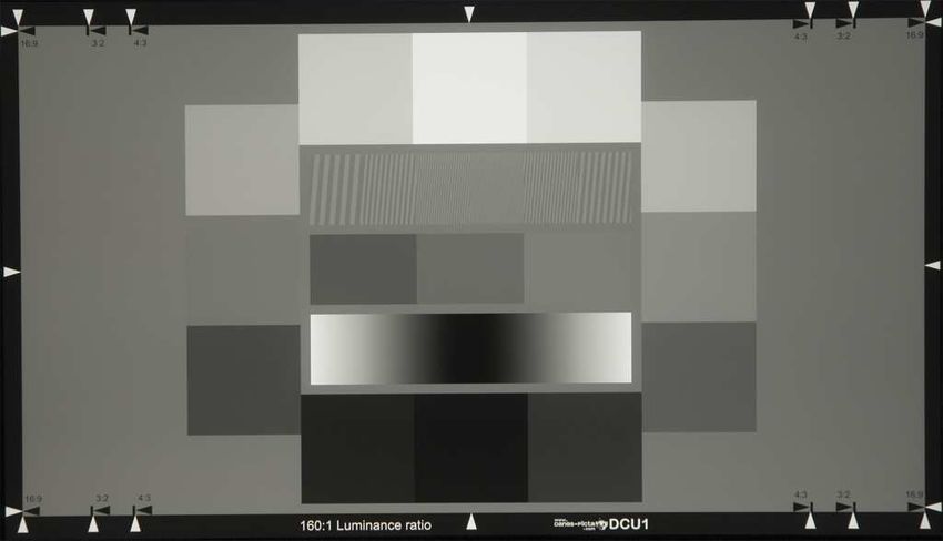
For noise and OECF measurements, there are two types of test charts used for, these are
transmissive and reflective. Transmissive test charts are partly transparent and shlould be
placed on light tables with constant luminance. Reflective test charts use light reflection.
In the case of this paper combined transmissive test chart with luminance ratio 160:1 [4] was
used for noise and OECF measurements, Fig 2(a). This chart is divided into 15 patches, their
placement is in Fig 2(b), where patches 1 - 12 are called OECF patches and patches 13 - 15 are
used for measurement of different noise types. Patch number 13 was used for purpose of basic
noise analysis.
(a) Transmissive test chart given by ISO 15739 (b) Patches placement in the transmissive test chart
Figure 2: Noise and OECF measurement test chart and patches placement, (a) Transmissive
test chart given by ISO 15739, (b) Patches placement in the transmissive test chart given by
ISO 15739
2.2 Noise type estimation
Estimate of noise PDF may be based on Pearson’s Chi-square test [5] or Kolmogorov-Smirnov
test [5], or both depending on used theoretical distribution. There were used patches 1-12 from
used test chart for purpose of noise type estimation. Following methods were applied to these
patches.Generalized Laplacian Model [7] (GLM) allows to model different types of probability
density functions and can also be used for noise type estimation. Its parameters are estimated
using method of moments. GLM is defined as
x p
e −| s |
p(x; s, p) = (10)
Z(s, p)
where s is band-width parameter of PDF, p is shape parameter, p ∈ h0, 1; 2, 5i and function
Z(s, p) is given as
µ 
s 1
Z(s, p) = 2 Γ . (11)
p p
Parameters in Eq. (10) can be estimated using moment methods, i.e., second and fourth cental
moments are then
³ ´ ³ ´ ³ ´
s2 Γ p3 s4 Γ 5
p Γ p
1
µ2 (s, p) = ³ ´ , µ4 (s, p) = ³ ´ . (12)
Γ p1 Γ p1
Combination of Eq. (12) leads to simplifying of GLM parameters estimation due to kurtosis
³ ´ ³ ´
5 1
µ4 (s, p) Γ p Γ p
κestimate = = ³ ´ . (13)
µ22 (s, p) Γ2 p3
Kurtosis using Eq. (13) is evaluated for all values p ∈ h0, 1; 2, 5i with chosen ∆p and then
compared with kurtosis evaluated from given data X. Value of κestimate closest to the value of κ
of given data, denotes the best estimate of para meter p. For normal distribution it is close
to value of 2. Band width parameter s with respect to µ4 (s, p) is then
v ³ ´
u
u Γ 1
u p
s = tµ2 ³ ´ . (14)
Γ p3
3 Noise analysis results
Nikon D40 SLR colour digital still camera with CCD sensor was analyzed with settings listed
• colour capture (single-chip RGB colour filter array camera),
• resolution of 6,1 milion of pixels,
• exposure time 1/200 s, 50 mm, lens set at f /5,6, ISO manual (ISO 200),
• no compression,
• log luminance values calculated from chart density measurements,
• fluorescent illumination, manual white balance.Similar settings were used for OECF and noise measurements. Size of analyzed cuts is 256 × 256
px. for OECF patches and 210 × 300 px. for patches 13a - 13c.
Fig. 3(a) and Fig. 3(b) show OECF of Nikon D40 digital still camera, digital output level and
log2 of digital output level vs. input log10 luminance for all (R, G, B) channels. OECF results
in tabular form are presented in Tab. 1.
(a) OECF Nikon D40 ISO−200, (b) OECF Nikon D40 ISO−200,
digital output level vs. input log luminance log of digital output level vs. input log luminance
10 2 10
220
R channel 7.5 R channel
200 G channel G channel
B channel 7 B channel
180
log of digital output level
160 6.5
digital output level
140 6
120
5.5
100
5
80
2
4.5
60
40 4
20 3.5
0.5 1 1.5 2 0.5 1 1.5 2
input log luminance input log luminance
10 10
Figure 3: (a) OECF - Nikon D40, ISO 200, digital output level vs. input log10 luminance, (b)
OECF - Nikon D40, ISO 200, log2 of digital output level vs. input log10 luminance
Table 1: OECF - Nikon D40, ISO 200
mean digital output levels
patch (step) log10 luminance
red green blue
1 0,27 9,78 9,83 9,81
2 0,71 20,34 20,27 20,19
3 1,04 39,77 39,68 39,05
4 1,30 55,66 55,70 53,84
5 1,52 79,80 79,80 78,09
6 1,70 102,06 102,21 99,76
7 1,87 124,88 124,89 122,95
8 2,01 147,30 147,29 145,29
9 2,14 166,48 166,49 164,97
10 2,26 185,43 185,60 184,11
11 2,37 202,72 203,32 202,70
12 2,47 221,55 222,73 221,64
Tab. 2 presents results of basic noise measurement for Nikon D40 using patch No. 13 given
by [4] and result camera noise is presented by σtotal [4] of patch No. 13b in this table, e.g.,
σtotal = 1, 49.
Table 2: Noise analysis of patch No. 13 - Nikon D40, ISO 200
patch No. σdiff σtemp σfp σtotal σave MCV
13a 0,67 0,69 0,99 1,72 1,01 71,55
13b 0,55 0,57 0,89 1,49 0,90 91,52
13c 0,46 0,47 0,63 1,10 0,65 110,10
Tab. 3 shows total, fixed-pattern and temporal SNR [4] of Nikon D40. Difference between
measured SNR and manufacturer may be given by the different evaluation method used by the
manufacturer.Table 3: SNR - Nikon D40, ISO 200
SNR type SN Rtotal SN Rfp SN Rtemp
measured value 41,82 70,07 108,46
manufacturer value 35,10 not available not available
Fig. 4 presents graphical form of σtotal , calculated according to [4], and σ gained as the simple
standard deviation in particular OECF patches.
Standard deviations in OECF patches, Nikon D40 ISO−200
4
sigma
3.5 σ by ISO 15739
total
3
2.5
σ, σtotal
2
1.5
1
0.5
0
1 2 3 4 5 6 7 8 9 10 11 12
patch No.
Figure 4: Standard deviations in OECF patches - Nikon D40, ISO 200
Tab. 4 presents noise standard deviations in OECF patches (columns 2 - 6) of analyzed test chart.
Column 8 of this table shows simple standard deviation in these patches from all acquired images
and column 7 contains mean code values (digital output levels) of particular patches.
Table 4: Standard deviations in OECF patches - Nikon D40, ISO 200
average σ given by ISO 15739
patch No. MCV σ
σdiff σtemp σfp σtotal σave
1 0,59 0,61 0,80 1,44 0,82 9,79 1,26
2 0,58 0,60 1,08 1,75 1,09 20,30 1,30
3 0,56 0,58 1,31 2,03 1,31 39,70 1,37
4 0,51 0,53 0,67 1,19 0,68 55,66 1,50
5 0,49 0,50 0,87 1,41 0,88 79,80 1,65
6 0,47 0,48 0,77 1,25 0,78 102,06 1,62
7 0,45 0,47 0,84 1,33 0,85 124,89 1,76
8 0,39 0,41 1,09 1,61 1,10 147,29 1,79
9 0,36 0,38 0,92 1,37 0,92 166,48 1,84
10 0,49 0,51 1,23 1,83 1,24 185,50 1,58
11 0,34 0,35 1,07 1,54 1,07 203,04 1,53
12 0,34 0,35 1,02 1,47 1,02 222,15 1,22
Standard deviations (variances) of σtotal and σ from particular OECF are 0,25 (0,06) and 0,18
(0,03), respectively. It means, that changes in both σtotal and σ are not so significant and it can
be considered, that the noise is signal independent.
Noise type estimation was based on PDF analysis of OECF patches histograms, all of them
presents Fig. 5.
Kolmogorov-Smirnov and χ2 test of goodness of fit were used for this purpose but they always
rejected the null hypothesis about tested distributions at used significance level, hence GLM
methods and kurtosis parameter were used for noise type estimation. Probability ditributions5 OECF patches histogram, Nikon D40 ISO−200
x 10
2.5
2
frequency
1.5
1
0.5
0
0 50 100 150 200 250
Figure 5: Histogram of OECF patches - Nikon D40, ISO 200
tested with used tests were Normal, Poisson, Erlang, Rayleigh and Exponential. Used signifi-
cance level of applied tests was α = 0.05.
Tab. 5 presents results for shape parameter p of GLM and kurtosis characteristic. It can be
seen, that p is mostly close or almost equal to value of 2 and kurtosis to value of 3. This leads
to the conclusion, that the noise is Normal.
Table 5: GLM shape parameter and kurtosis values - Nikon D40, ISO 200
Patch No. 1 2 3 4 5 6 7 8 9 10 11 12
GLM shape
1,94 2,19 2,23 1,85 1,74 2,02 1,96 2,50 1,94 1,78 2,50 2,50
param. p
kurtosis κ 3,07 2,84 2,80 3,18 3,32 2,97 3,04 2,63 3,07 3,32 2,62 2,61
4 Conclusion
The main goal of this paper was to acquire set of test images using Nikon D40 digital still
camera and evalute noise characteristics such as standard deviation and SNR, determine noise
dependence on input luminance level and its probability distribution. Value of SN Rtotal of tested
camera using sensitivity ISO 200 was determined as 41,82. These value does not correspond
to the value given by the manufacturer for reference signal level of 18 % but match to reference
signal level of 100 %. These differences may be caused by different measuring methods that are
used by the manufacturer and defined in used ISO standard. When we discus dependency of noise
level on input luminance level, then it is possible to say that the noise is signal independent,
because standard deviations of σtotal and σ from particular OECF patches are insignificant,
Fig. 4. In the case of analyzed camera it is 0,25 for σtotal and 0,18 for σ. OECF of tested system
is not linear, Fig. 3(b), which can cause difficulties during restoration of images acquired by this
camera.
Probability distributions were tested with statistical hypothesis tests, χ2 test of goodness of fit
and Kolmogorov-Smirnov test but neither test proved any of tested distributions. Thus there
were used shape parameter of GLM and kurtosis to determine noise distribution. From results,
Tab. 5, can be seen that shape parameters are close to value of 2 and kurtosis to values of 3,
which corresponds to the Normal distribution and thus the noise distribution can be considered
as Gaussian in whole spectrum of grayscale.References
[1] Ajoy K. R. Acharya T. Image Processing: Principles and Applications. Jonh Wiley & Sons
Inc., U.S.A., 2005.
[2] Bijaoui A. Starck J. L., Murtagh F. Image processing and data analysis: The multiscale
approach. Cambridge University Press, Cambridge, U.K., first edition, 1998.
[3] International standard ISO 14524:1999(E). ISO copyright office, http://www.iso.org, 1999.
[4] International standard ISO 15739:2003(E). ISO copyright office, http://www.iso.org, 2003.
[5] Pavlı́k J., a kol. Applied statistics. ICT, Prague, CZ, first edition, 2005.
[6] Saeed V. Vaseghi. Advanced Digital Signal Processing and Noise Reduction. John Wiley &
Sons Ltd., U.K., third edition, 2006.
[7] Simoncelli E. P, Adelson E. H.: Noise removal via Bayesian wavelet coring. International
Conference on Image Processing (ICIP-96), 16-19 September 1996, Vol. I, pp. 379-382.
[8] Woods E. R. Gonzalez C. R. Digital Image Processing. Prentice Hall, U.S.A., second edition
edition, 2002.
František Mojžı́š
Department of Computing and Control Engineering
Institute of Chemical Technology in Prague
Technická 5, 166 28 Prague 6, Czech republic
E-mail: frantisek.mojzis@vscht.cz
Jan Švihlı́k
Department of Computing and Control Engineering
Institute of Chemical Technology in Prague
Technická 5, 166 28 Prague 6, Czech republic
E-mail: jan.svihlik@vscht.czYou can also read