Noise Estimation Is Not Optimal: How to Use Kalman Filter the Right Way
←
→
Page content transcription
If your browser does not render page correctly, please read the page content below
Noise Estimation Is Not Optimal:
                                                      How to Use Kalman Filter the Right Way

                                                     Ido Greenberg                  Netanel Yannay                 Shie Mannor
                                             Department of Electric Engineering,                          Department of Electric Engineering,
                                                     Technion, Israel                                             Technion, Israel
arXiv:2104.02372v3 [cs.LG] 20 May 2021

                                              gido@campus.technion.ac.il                                          Nvidia Research

                                                                                       Abstract
                                                   Determining the noise parameters of a Kalman Filter (KF) has been studied for
                                                   decades. A huge body of research focuses on the task of estimation of the noise
                                                   under various conditions, since precise noise estimation is considered equivalent to
                                                   minimization of the filtering errors. However, we show that even a small violation
                                                   of the KF assumptions can significantly modify the effective noise, breaking the
                                                   equivalence between the tasks and making noise estimation an inferior strategy.
                                                   We show that such violations are very common, and are often not trivial to handle
                                                   or even notice. Consequentially, we argue that a robust solution is needed – rather
                                                   than choosing a dedicated model per problem. To that end, we apply gradient-based
                                                   optimization to the filtering errors directly, with relation to a simple and efficient
                                                   parameterization of the symmetric and positive-definite parameters of KF. In radar
                                                   tracking and video tracking, we show that the optimization improves both the
                                                   accuracy of KF and its robustness to design decisions. In addition, we demonstrate
                                                   how an optimized neural network model can seem to reduce the errors significantly
                                                   compared to a KF – and how this reduction vanishes once the KF is optimized
                                                   similarly. This indicates how complicated models can be wrongly identified as
                                                   superior to KF, while in fact they were merely more optimized.

                                         1     Introduction
                                         The Kalman Filter (KF) [Kalman, 1960] is a celebrated method for linear filtering and prediction,
                                         with applications in many fields including tracking, guidance, navigation and control [Zarchan and
                                         Musoff, 2000, Kirubarajan, 2002]. Due to its simplicity and robustness, it remains highly popular
                                         – with over 10,000 citations in the last 5 years alone [Google Scholar, 2021] – despite the rise of
                                         many non-linear sequential prediction models (e.g., recurrent neural networks). The KF relies on the
                                         following model for a dynamic system:
                                                                        Xt+1 = F Xt + ωt         (ωt ∼ N (0, Q))
                                                                                                                                              (1)
                                                                          Zt = HXt + νt          (νt ∼ N (0, R))
                                         where Xt is the (unknown) state of the system at time t, whose dynamics are modeled by the linear
                                         operator F up to the random noise ωt with covariance Q; and Zt is the observation, which is modeled
                                         by the linear operator H up to the noise νt with covariance R.
                                         Many works have addressed the challenge of determining the noise parameters Q, R [Abbeel et al.,
                                         2005, Odelson et al., 2006, Zanni et al., 2017, Park et al., 2019]. Since the KF yields minimal errors
                                         when Q and R correspond to the true covariance matrices of the noise [Humpherys et al., 2012], these
                                         parameters are usually determined by noise estimation. This is particularly true when the training data
                                         contain the ground-truth (i.e., the system states), in which case the noise can be trivially estimated by
                                         the sample covariance matrix. Other methods are needed in absence of the ground-truth, but as stated

                                         Preprint. Under review.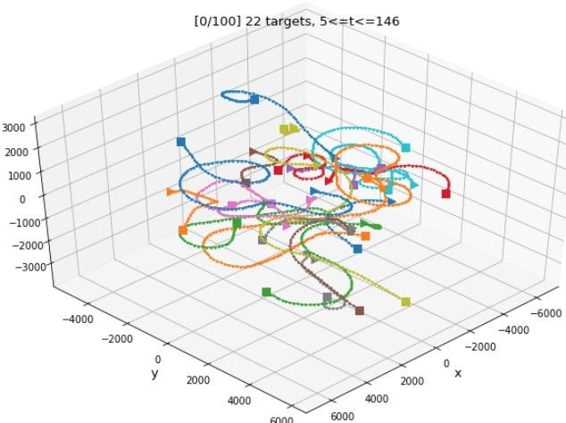
by Odelson et al. [2006], “the more systematic and preferable approach to determine the filter gain
is to estimate the covariances from data”. This work focuses on such problems with ground-truth
available for learning (but not for inference after the learning, of course), which was motivated by a
real-world Doppler radar estimation problem.

Noise estimation is not optimal: The equivalence between noise estimation and errors minimiza-
tion can be proved under the standard assumptions of KF – that is, known and linear dynamics and
observation models (F, H), with i.i.d and normally-distributed noises ({ωt }, {νt }) [Humpherys et al.,
2012]. However, as put by Thomson [1994], “experience with real-world data soon convinces one
that stationarity and Gaussianity are fairy tales invented for the amusement of undergraduates” – and
linearity and independence can be safely added to this list. Therefore, under realistic assumptions,
the covariance of the noise does not necessarily correspond to optimal filtering.
We introduce a case study in the context of radar tracking, where we demonstrate that even using
the exact covariance of the noise ("oracle-based" parameters) is highly sub-optimal – even in very
simplistic scenarios with relatively minor violation of KF assumptions. We analyze this phenomenon
analytically for the case of non-linear observation model in a Doppler radar, where the violation
of linearity is shown to modify the effective noise. By providing this extensive evidence for the
sub-optimality of noise estimation in practical applications of the KF, we re-open a problem that
was considered solved for decades [Kalman, 1960].
We also show that seemingly small changes in the properties of the scenario sometimes lead to major
changes in the desired design of the KF, e.g., whether to use a KF or an Extended KF [Julier and
Uhlmann, 2004]. In certain cases, the design choices are easy to overlook (e.g., Cartesian vs. polar
coordinates), and are not trivial to make even if noticed. As a result, it is impractical to manually
choose or develop a variant of KF for every problem. Rather, we should assume that our model is
sub-optimal, and leverage data to deal with the sub-optimality as robustly as possible.

How to use KF the right way: We consider Q and R as model parameters that should be optimized
with respect to the filtering errors – rather than estimating the noise. While both noise estimation and
errors optimization rely on exploitation of data, only the latter explicitly addresses the actual goal of
solving the filtering problem.
Many gradient-based optimization methods have been demonstrated effective in the field of machine
learning, but applying them naively to the entries of Q and R may violate the symmetry and positive-
definiteness (SPD) constraints of the covariance matrices. Indeed, even works that come as far as
optimizing Q and R (instead of estimating the noise) usually apply limited optimization methods, e.g.,
grid-search [Coskun et al., 2017] or diagonal restriction of the covariance matrices [Formentin and
Bittanti, 2014, Li et al., 2019]. To address this issue, we use a parameterization based on Cholesky
decomposition [Horn and Johnson, 1985], which allows us to apply gradient-based optimization to
SPD matrices. This method is computationally efficient compared to other general gradient-based
methods for SPD optimization [Tsuda et al., 2005, Tibshirani, 2015].
We demonstrate that the optimization reduces the errors of KF consistently: over different variants
of KF, over different scenarios of radar tracking, and even in the different domain of tracking from
video. In most cases, the likelihood score of the tracker is improved as well, which is important
for matching of observations to targets in the multi-target tracking problem. Furthermore, we show
that optimization improves the robustness to design decisions, by shrinking the gaps between the
performance of different variants of KF. We also demonstrate that optimization generalizes well under
distributional shifts between train and test data, and in that sense does not overfit the train data more
than noise estimation.
As explained above, we extensively justify the need to optimize KF in almost any practical problem,
and suggest a simple solution that is effective, robust, computationally efficient, and relies on standard
tools in supervised machine learning. As a result, we believe that in the scope of filtering problems
with available ground-truth, the suggested optimization method is capable of becoming the new
standard procedure for tuning of KF.

Unfair comparison: Many learning algorithms have been suggested to address non-linearity in
filtering problems, e.g., based on Recurrent Neural Networks (RNN). Such works often use a linear
tool such as the KF as a baseline for comparison – with tuning parameters being sometimes ignored

                                                    2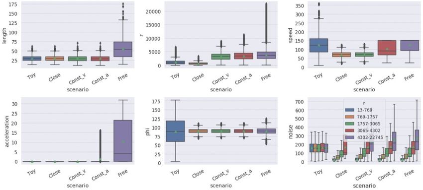
[Gao et al., 2019], sometimes based on noise estimation [fa Dai et al., 2020], and sometimes optimized
in a limited manner using trial-and-error [Jamil et al., 2020] or grid-search [Coskun et al., 2017]. Our
findings imply that such a methodology yields over-optimistic conclusions, since the baseline is not
optimized to the same level as the learning model. This may result in adoption of over-complicated
algorithms with no actual added value. Instead, any learning algorithm should be compared to a
baseline that is optimized using a similar method (e.g., gradient-descent with respect to the errors).
Indeed, we consider an extension of KF based on LSTM, which is the key component in most
SOTA algorithms for non-linear sequential prediction in recent years [Neu et al., 2021]. For radar
tracking with non-linear motion, we demonstrate how the LSTM seems to provide a significant
improvement over the KF. Then, we show that the whole improvement comes from optimization of
parameters, and not from the expressive non-linear architecture. In particular, this result demonstrates
the competitiveness of our suggested method versus SOTA sequential prediction models.
Recent works in the area of machine learning have already shown that advanced algorithms often
obtain most of their improvement from implementation nuances [Engstrom et al., 2019, Andrychowicz
et al., 2020, Henderson et al., 2017]. Our work continues this line of thinking and raises awareness to
this issue in the domain of filtering problems, in order to enhance the value of existing algorithms,
and avoid unnecessarily complicated and costly ones.

Contribution: We show that KF is used incorrectly in a variety of problems; show that advanced
filtering algorithms are often tested unfairly; suggest a simple method to solve both issues, using
gradient-based optimization along with Cholesky decomposition; and provide a detailed case study
that analyzes the differences between noise estimation and parameters optimization empirically and
(for a specific benchmark) analytically.
The paper is organized as follows: Section 2 reviews KF and RNN. Section 3 demonstrates the
necessity of optimization in KF through a detailed case study. Section 4 introduces our method for
efficient optimization of KF parameters. Section 5 presents a neural version of KF which reduces the
errors compared to a standard KF – but not when compared to an optimized KF. Section 6 discusses
related works, and Section 7 summarizes.

2   Preliminaries and Problem Setup
Kalman Filter: The KF algorithm relies on the model of Eq. (1) for a dynamic system. It keeps an
estimate of the state Xt , represented as the mean xt and covariance Pt of a normal distribution. As
shown in Figure 1, it alternately predicts the next state using the dynamics model (prediction step),
and processes new information from incoming observations (update or filtering step).
While being useful and robust, KF
yields optimal estimations only un-
der a restrictive set of assump-
tions [Kalman, 1960], as specified in
Definition 2.1.
Definition 2.1 (KF assumptions).
F, H of Eq. (1) are constant and
known matrices; ωt , νt are i.i.d ran-
dom variables with zero-mean and
constant, known covariance matrices
Q, R, respectively; and the distribu-
tion of the random initial state X0 is
known.                                 Figure 1: A diagram of the KF algorithm. Note that the prediction
                                         step is based on the motion model F with noise Q, whereas the
Note that both motion and observation update step is based on the observation model H with noise R.
models in Definition 2.1 are assumed
to be linear, and both sources of noise are i.i.d with known covariance. Normality of the noise is also
often assumed, but is not necessary for optimality [Humpherys et al., 2012].
Violations of some of the assumptions in Definition 2.1 can be handled by certain variations of the
KF, such as the Extended KF (EKF) [Julier and Uhlmann, 2004] which replaces the linear models
F, H with local linear approximations, and the Unscented KF (UKF) [Wan and Van Der Merwe,

                                                   3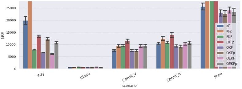
2000] which applies particle-filtering approach. The use of multiple tracking models alternately is
also possible using switching mechanisms [Mazor et al., 1998].
While F and H are usually determined based on domain knowledge, Q and R are often estimated
from data as the covariance of the noise. Many works consider the problem of estimation from
the observations alone, but when the true states are available in the data, the estimation becomes a
straight-forward computation of the sample covariance matrices [Lacey, 1998]:
                     R̂ := Cov({zt − Hxt }t ),          Q̂ := Cov({xt+1 − F xt }t ).                   (2)

Recurrent neural networks: A RNN [Rumelhart et al., 1986] is a neural network that is intended
to be iteratively fed with sequential data samples, and that passes information (the hidden state) over
iterations. Every iteration, the hidden state is fed to the next copy of the network as part of its input,
along with the new data sample. Long Short Term Memory (LSTM) [Hochreiter and Schmidhuber,
1997] is an architecture of RNN that is particularly popular due to the linear flow of the hidden state
over iterations, allowing it to capture memory for relatively long term. The parameters of a RNN are
usually optimized in a supervised manner with respect to a training dataset of input-output pairs.
For a more detailed introduction of the preliminaries, see Appendix A.

3     Kalman Filter Configuration and Optimization: a Case Study
In this section, we compare noise estimation and errors optimization in KF through a detailed case
study. Once we understand the importance of optimization in KF, Section 4 discusses its challenges
and suggests an efficient optimization method under the constraints of KF.
The performance of a KF strongly depends on its parameters Q and R. These parameters are
usually regarded as estimators of the noise covariance in motion and observation, respectively [Lacey,
1998], and are estimated accordingly. Even though optimization has been suggested for KF in the
past [Abbeel et al., 2005], it was often viewed as a fallback solution [Odelson et al., 2006], for cases
where direct estimation is not possible (e.g., the true states are unavailable in the data [Feng et al.,
2014]), or where the problem is more complicated (e.g., non-stationary noise [Akhlaghi et al., 2017]).
The preference of estimation relies on the fact that KF – with parameters corresponding to the
noise covariances – provides optimal filtering errors. However, the optimality only holds under the
assumptions specified in Definition 2.1 [Humpherys et al., 2012]. Some of these assumptions are
clearly violated in realistic scenarios, while other violations may be less obvious. For example, even
if a radar’s noise is i.i.d in polar coordinates, it is not so in Cartesian coordinates (see Appendix A.4).
The need to rely on many assumptions might explain why there are several extensions and design deci-
sions in the configuration of a KF. This includes the choice between KF and EKF [Julier and Uhlmann,
2004]; the choice between educated state initialization and a simple uniform prior [Linderoth et al.,
2011]; and certain choices that may be made without even noticing, such as the coordinates of the
state representation.
The case study below justifies the following claims:
       1. The design decisions in KF are often nontrivial to make and are potentially significant.
       2. Tuning KF by noise estimation is often highly sub-optimal – even in very simple scenarios.
       3. Tuning KF by optimization improves both accuracy and robustness to design decisions.
These claims mean that the popular KF algorithm is often not exploited to its full potential. Further-
more, many works that compare learning algorithms to a KF baseline conduct an "unfair" comparison,
as the learning algorithms are optimized and the KF is not. This may lead to adoption of unnecessarily
complicated algorithms, as demonstrated in Section 5. Indeed, in many works the tuning of the
baseline KF is either ignored in the report [Gao et al., 2019] or relies on noise estimation [fa Dai
et al., 2020], sometimes directly by the observing sensor [Jamil et al., 2020].

3.1   Setup and methodology

In the case study of the radar tracking problem, each target is represented by a sequence of (unknown)
states in consecutive time-steps, and a corresponding sequence of radar measurements. A state

                                                    4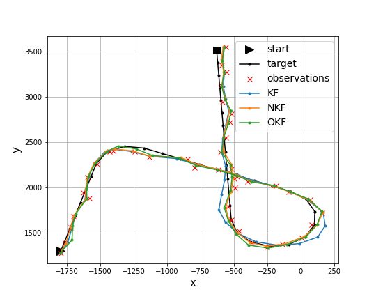
xf ull = (xx , xy , xz , xvx , xvy , xvz )> ∈ R6 consists of 3D location and velocity. We also denote
x = (xx , xy , xz )> ∈ R3 for the location alone (or xtarget,t ∈ R3 for the location of a certain target
at time t). An observation z ∈ R4 consists of noisy measurements of range, azimuth, elevation
and Doppler signal. Note that the former three correspond to a noisy measurement of x in polar
coordinates, and the latter one measures the projection of velocity onto the radial direction x.
The task of interest is estimation of xtarget,t at anyPt. Denoting the corresponding point-estimate by
x̃target,t , our primary goal is to minimize M SE = target t (x̃target,t −xtarget,t )2 . As a secondary goal,
P
P
P P
we also wish to minimize the negative-log-likelihood N LL = − target t log l(xtarget,t Dtarget,t ).
P
Here Dtarget,t is the distribution of the target location at time t, predicted using observations up to
time t − 1 (i.e., in terms of the KF, after the prediction step at time t − 1), and l is the corresponding
likelihood. While our case study focuses on tracking a single target at a time, N LL minimization is
useful for matching observations to targets in the scope of the multi-target tracking problem.
The case study considers 5 types of tracking scenarios (benchmarks) and 4 variants of KF (baselines).
For each benchmark and each baseline, we use the training data of the benchmark to produce one KF
model with estimated noise parameters (Eq. (2)) and one with optimized parameters (see Section 4).
We then evaluate the errors of both models on the test data of the benchmark (generated using different
seeds than the training data). All experiments were run on eight i9-10900X CPU cores on a single
Ubuntu machine.
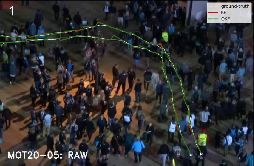
Figures 2b,2c display a sample of trajectories in the simplest benchmark (Toy), which satisfies
all KF assumptions except for a linear observation model H; and in the Free Motion benchmark,
which violates several assumptions (in a similar complexity as the scenario of Section 5). The other
benchmarks are demonstrated in Appendix G. Figure 2a defines each of the 5 benchmarks more
formally as a certain subset of the following properties:
• anisotropic: horizontal motion is more likely than vertical motion (otherwise motion direc-
tion is distributed uniformly).
• polar: radar noise is generated i.i.d in polar coordinates (otherwise noise is Cartesian i.i.d,
which violates the physics of the system).
• uncentered: targets are not forced to concentrate close to the radar.
• acceleration: speed change is allowed.
• turns: non-straight motion is allowed.
(a) (b) (c)
Figure 2: (a) Benchmarks names (rows) and the properties that define them (columns). Green means that the
benchmark satisfies the property. (b,c) Samples of trajectories (projected onto XY plane) in Toy benchmark and
Free Motion benchmark.
The 4 baselines differ from each other by using either KF or EKF, with either Cartesian or
polar coordinates for representation of R (the rest of the system is always represented in Cartesian
coordinates). In addition, as mentioned above, each baseline is tuned once by noise estimation and
once by parameters optimization. See Appendix B for more details about the experimental setup.
We also repeat the experiment for the problem of tracking from video, using MOT20 dataset [Dendor-
fer et al., 2020] of real-world pedestrians, with train and test datasets taken from separated videos.
For this problem we only consider a KF with Cartesian coordinates, since there is no polar component
in the problem. Note that in contrast to radar tracking, video tracking enjoys a perfectly linear
5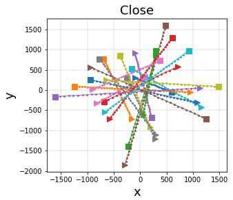
Table 1: Summary of the out-of-sample errors of the various models over the various benchmarks. In the names
of the models, "O" denotes optimized, "E" denotes extended, and "p" denotes polar (e.g., OEKFp is an extended
KF with polar representation of R and optimized parameters). For each benchmark, the best estimated model
and the best optimized model are marked. For KFp, we also consider an oracle-realization of R according to the
true noise of the simulated radar in polar coordinates (available only in polar benchmarks). Note that (1) for any
benchmark and any baseline, optimization yields lower error than estimation; and (2) this remains true even in
the oracle variant, where the noise estimation is perfect.
 Benchmark KF              OKF      KFp       KFp (oracle)     OKFp EKF OEKF                 EKFp      OEKFp
    Toy    151.7           84.2     269.6          –           117.4 92.8   79.3             123.0      109.1
   Close    25.0           24.9      22.6        22.5           22.5  26.4  26.2              24.5       24.1
  Const_v   90.2           90.0     102.3       102.3           89.3 102.5 101.5             112.7      102.2
  Const_a  107.5           101.7    118.4       118.3          100.5 110.0 107.5             126.0      108.9
    Free   125.9           118.8    145.6       139.3          118.1 135.8 122.1             149.3      120.2

observation model. This extends the scope of the experiments in terms of KF assumptions violations.
See Appendix E for the detailed setup of the video tracking experiments.

3.2   Results

Design decisions are not trivial: Table 1 summarizes the tracking errors. The left column in
each cell corresponds to a model with estimated (not optimized) parameters, and shows that in each
benchmark, the errors strongly depend on the design decisions (R’s coordinates and whether to use
EKF). In Toy benchmark, for example, EKF is the best design, since the observation model H is
non-linear.
However, in other benchmarks the winning designs are arguably surprising:

      1. Under non-isotropic motion direction, EKF is worse than KF in spite of the non-linear
         motion. It is possible that since the horizontal prior reduces the stochasticity of H, the
         advantage of EKF no longer justifies the instability of the derivative-based approximation.
      2. Even when the observation noise is polar i.i.d, polar representation of R is not beneficial
         unless the targets are forced to concentrate close to the radar. It is possible that when
         the targets are distant, Cartesian coordinates have a more important role in expressing the
         horizontal prior of the motion.

Since the best variant of KF for each benchmark seems difficult to predict in advance, a practical
system cannot rely on choosing the KF variant optimally, and rather has to be robust to this choice.

Optimization is both beneficial and robust: Table 1 shows that for any benchmark and any
baseline, parameters optimization yielded smaller errors than noise estimation (over an out-of-sample
test dataset). In addition, the variance between the baselines reduces under optimization, i.e., the
optimization makes KF more robust to design decisions (which is also evident in Figure 9a in
Appendix G).
We also studied the performance of a KF with a perfect
knowledge of the noise covariance matrix R. Note that
in the constant-speed benchmarks, the estimation of Q =
0 is already very accurate, hence in these benchmarks
the oracle-KF has a practically perfect knowledge of
both noise covariances. Nonetheless, Table 1 shows
that the oracle yields very similar results to a KF with
estimated parameters. This indicates that the limitation
of noise estimation in KF indeed comes from choosing
the wrong goal, and not from estimation inaccuracy.
Figure 3 shows that parameters optimization provides
significantly better predictions also in tracking from Figure 3: Prediction errors of KF and OKF on
video, where it reduces the MSE by 18% (see Ap- 1208 targets of the test data of MOT20 videos
pendix E for more details).                            dataset. OKF is significantly more accurate.

                                                        6
Diagnosis of KF sub-optimality in Toy scenario: The source of the gap between estimated and
optimized noise parameters can be studied through the simplest Toy benchmark, where the only
violation of KF assumptions is the non-linear observation model H. Since the non-constant entries
of H correspond to the Doppler observation, the non-linearity inserts uncertainty to the Doppler
observation (in addition to the inherent observation noise). This increases Doppler’s effective noise
in comparison to the location observation, as shown analytically in Appendix D. This explanation is
consistent with Figure 4: the noise associated with Doppler is indeed increased by the optimization.

4   Optimization of SPD Matrices Using Cholesky Decomposition

As explained in Section 3, Q and R are usu-
ally considered as estimators of the noise. Even
when viewed as parameters to optimize with
respect to the filtering errors, they are still of-
ten determined by trial-and-error or by a grid-
search [Formentin and Bittanti, 2014, Coskun
et al., 2017]. The experiments in Section 3,
however, required a more systematic optimiza-
                                                         (a) Estimated R            (b) Optimized R
tion. To that end, we chose the Adam algo-
rithm [Diederik P. Kingma, 2014], with respect Figure 4: The covariance matrix R of the observation
to a loss function consisting of a linear combina- noise obtained in a (Cartesian) KF by noise estimation
tion of the squared filtering errors (MSE) and the and by optimization, based on the dataset of the Toy
negative log likelihood (NLL). Adam is a pop- benchmark. Note that the noise estimation is quite ac-
ular variant of the well-known gradient-descent curate for this 2
                                                                  benchmark, as the true variance of the
                                                                                                    2
algorithm, and has achieved remarkable results noise is 100 for the positional dimensions and 5 for
in many optimization problems in the field of the Doppler signal.
machine learning in recent years, including in non-convex problems where local-minima exist.
Unfortunately, Adam cannot be applied directly to the entries of Q and R without ruining the
symmetry and positive definiteness (SPD) properties of the covariance matrices. This difficulty often
motivates optimization methods that avoid gradients [Abbeel et al., 2005], or even the restriction
of Q and R to be diagonal [Li et al., 2019]. Indeed, Formentin and Bittanti [2014] pointed out that
“since both the covariance matrices must be constrained to be positive semi-definite, Q and R are
often parameterized as diagonal matrices”.
To allow Adam to optimize the non-diagonal Q and R we use the Cholesky decomposition [Horn and
Johnson, 1985], which states that any SPD matrix A ∈ Rn×n can be written as A = LL> , where
L is lower-triangular with positive entries along its diagonal. The reversed claim is also true: for
any lower-triangular L with positive diagonal, LL> is SPD. Now consider the parameterization of A
using the following n2 + n = n(n+1)    parameters: n2 parameters correspond to {Lij }1≤j is continuous and outputs a SPD matrix for any realization of the parameters
in Rn(n+1)/2 . Thus, we can apply Adam [Diederik P. Kingma, 2014] (or any other gradient-based
method) to optimize these parameters without worrying about the SPD constraints. This approach,
which is presented more formally in Appendix F and implemented in our code, was used for all the
KF optimizations in this work.
The parameterization of covariance matrices using Cholesky decomposition was already suggested by
Pinheiro and Bates [1996]. However, despite its simplicity, it is not commonly used for gradient-based
optimization in SPD matrices in general, and to the best of our knowledge is not used at all for
optimization of KF parameters in particular. Other methods were also suggested for SPD optimization,
e.g., matrix-exponent [Tsuda et al., 2005] and projected gradient-descent with respect to the SPD
cone [Tibshirani, 2015]. These methods require SVD-decomposition in every iteration, hence are
computationally heavy, which may explain why they are not commonly used for tuning of KF. The
parameterization derived from Cholesky decomposition only requires a single matrix multiplication,
and thus is both efficient and easy to implement.
In addition to its efficiency, the suggested method is shown in Section 3 to be both effective and
robust in tuning of KF. Furthermore, as it relies on standard tools from supervised machine learning,
it is also applicable to high-dimensional parameters spaces. Consequentially, we believe that this

                                                   7
method is capable of replacing noise estimation as the standard method for KF parameters tuning, in
the scope of filtering problems with presence of ground-truth training data.
5 Neural Kalman Filter: Is the Non-linear Prediction Helpful?
A standard Kalman Filter for a tracking task assumes linear motion, as discussed in Section 2.
In this section we introduce the Neural Kalman Filter tracking model (NKF), which uses LSTM
networks to model non-linear motion, while keeping the framework of KF – namely, the probabilistic
representation of the target’s state, and the separation between prediction and update steps.
Every prediction step, NKF uses a neural network model to predict the target’s acceleration at and
the motion uncertainty Qt . Every update step, another network predicts the observation uncertainty
Rt . The predicted quantities are incorporated into the standard update equations of KF, which are
stated in Figure 1. For example, the prediction step of NKF is:
xP
t+1 = F xt + 0.5at (∆t)
2
P
Pt+1 = F Pt F > + Qt
where F = F (∆t) is the constant-velocity motion operator, and at , Qt are predicted by the LSTM
(whose input includes the recent observation and the current estimated target’s state). Other predictive
features were also attempted but failed to provide significant value, as described in Appendix B. Note
that the neural network predicts the acceleration rather than directly predicting the location. This is
intended to regularize the predictive model and to exploit the domain knowledge of kinematics.
After training NKF over a dataset of simulated targets with random turns and accelerations (see
Appendix B for more details), we tested it on a separated test dataset. The test dataset is similar to
the training dataset, with different seeds and an extended range of permitted accelerations. As shown
in Figure 5, NKF significantly reduces the tracking errors compared to a standard KF.
(a) (b)
Figure 5: (a) Relative tracking errors (lower is better) with relation to a standard KF, over targets with different
ranges of acceleration. The error-bars represent confidence intervals of 95%. The label of each bar represents
the corresponding absolute MSE (×103 ). In the training data, the acceleration was limited to 24-48, hence the
other ranges measure generalization. While the Neural KF (NKF) is significantly better than the standard KF, its
advantage is entirely eliminated once we optimize the KF (OKF). (b) A sample target and the corresponding
models outputs (projected onto XY plane). The standard KF has a difficulty to handle some of the turns.
At this point, it seems that the non-linear architecture of NKF provides a better tracking accuracy in
the non-linear problem of radar tracking. However, Figure 5 shows that by shifting the baseline from
a naive KF to an optimized one, we completely eliminate the advantage of NKF, and in fact reduce
the errors even further. In other words, the benefits of NKF come only from optimization and not at
all from the expressive architecture. Hence, by overlooking the sub-optimality of noise estimation in
KF, we would wrongly adopt the over-complicated model of NKF.
Note that the optimized variant of KF also generalizes quite well to targets with different accelerations
than observed in the training. This indicates a certain robustness of the optimized KF to distributional
shifts between the train and test data. Also note that while Figure 5 summarizes tracking errors,
Figure 8 in Appendix G shows that the likelihood of the model is also improved by the optimized KF.
High likelihood is important for the matching task in a multi-target tracking problem.
86 Related Work
Noise estimation: Estimation of the noise parameters in KF has been studied for decades. A
popular framework for this problem is estimation from data of observations alone [Odelson et al.,
2006, Feng et al., 2014, Park et al., 2019], since the ground-truth of the states is often unavailable in
the data [Formentin and Bittanti, 2014]. In this work we assume that the ground-truth is available,
where the current standard approach is to simply estimate the noise covariance matrix from the
data [Odelson et al., 2006].
Many works addressed the problem of non-stationary noise estimation [Zanni et al., 2017, Akhlaghi
et al., 2017]. However, as demonstrated in Sections 3,5, in certain cases stationary methods are highly
competitive if tuned correctly – even in problems with complicated dynamics.
Optimization: In this work we apply gradient-based optimization to KF with respect to its errors.
An optimization method that avoids gradients computation was already suggested in Abbeel et al.
[2005]. In practice, "optimization" of KF is often handled manually using trial-and-error [Jamil et al.,
2020], or using a grid-search over possible values of Q and R [Formentin and Bittanti, 2014, Coskun
et al., 2017]. In other cases, Q and R are restricted to be diagonal [Li et al., 2019, Formentin and
Bittanti, 2014].
Gradient-based optimization of SPD matrices in general was suggested in Tsuda et al. [2005]
using matrix-exponents, and is also possible using projected gradient-descent [Tibshirani, 2015] –
both rely on SVD-decomposition. In this work, we apply gradient-based optimization using the
parameterization that was suggested in Pinheiro and Bates [1996], which requires a mere matrix
multiplication, and thus is both efficient and easy to implement.
Neural networks in filtering problems: Section 5 presents a RNN-based extension of KF, and
demonstrates how its advantage over the linear KF vanishes once the KF is optimized. The use of
neural networks for non-linear filtering problems is very common in the literature, e.g., in online
tracking prediction [Gao et al., 2019, Dan Iter, 2016, Coskun et al., 2017, fa Dai et al., 2020, Ullah
et al., 2019], near-online prediction [Kim et al., 2018], and offline prediction [Liu et al., 2019b].
In addition, while Bewley et al. [2016] apply a KF for video tracking from mere object detections,
Wojke et al. [2017] add to the same system a neural network that generates visual features as well.
Neural networks were also considered for related problems such as data association [Liu et al., 2019a],
model-switching [Deng et al., 2020], and sensors fusion [Sengupta et al., 2019].
In many works that consider neural networks for filtering problems, a variant of the KF is used
as a baseline for comparison. However, while the parameters of the neural networks are normally
optimized to minimize the filtering errors, the parameters tuning of the KF is sometimes ignored [Gao
et al., 2019], sometimes based on noise estimation [fa Dai et al., 2020], and sometimes optimized in a
limited manner as mentioned above [Jamil et al., 2020, Coskun et al., 2017]. Our findings imply that
such a methodology yields over-optimistic conclusions, since the baseline is not optimized to the
same level as the learning model.
See Appendix C for an extended discussion on related works.
7 Summary
Through a detailed case study, we demonstrated both analytically and empirically how fragile are
the assumptions of the KF, and how the slightest violation of them may change the effective noise
in the problem – leading to significant changes in the optimal noise parameters. We addressed this
problem using optimization tools from supervised machine learning, and suggested how to apply
them efficiently to the SPD parameters of KF. As this method was demonstrated accurate and robust
in both radar tracking and video tracking, we recommended to use it as the default procedure for
tuning of KF in presence of ground-truth data.
We also demonstrated one of the consequences of the use of sub-optimal KF: the common methodol-
ogy of comparing learning filtering algorithms to classic variants of KF is misleading, as it essentially
compares an optimized model to a non-optimized one. We argued that the baseline method should be
optimized similarly to the researched one, e.g., using the optimization method suggested in this work.
9References
Pieter Abbeel, Adam Coates, Michael Montemerlo, Andrew Ng, and Sebastian Thrun. Discriminative
training of kalman filters. Robotics: Science and systems, pages 289–296, 06 2005. doi: 10.15607/
RSS.2005.I.038.
S. Akhlaghi, N. Zhou, and Z. Huang. Adaptive adjustment of noise covariance in kalman filter for
dynamic state estimation. In 2017 IEEE Power Energy Society General Meeting, pages 1–5, 2017.
doi: 10.1109/PESGM.2017.8273755.
Marcin Andrychowicz, Anton Raichuk, Piotr Stańczyk, Manu Orsini, Sertan Girgin, Raphael Marinier,
Léonard Hussenot, Matthieu Geist, Olivier Pietquin, Marcin Michalski, Sylvain Gelly, and Olivier
Bachem. What matters in on-policy reinforcement learning? a large-scale empirical study, 2020.
S. T. Barratt and S. P. Boyd. Fitting a kalman smoother to data. In 2020 American Control Conference
(ACC), pages 1526–1531, 2020. doi: 10.23919/ACC45564.2020.9147485.
Alex Bewley, Zongyuan Ge, Lionel Ott, Fabio Ramos, and Ben Upcroft. Simple online and realtime
tracking. In 2016 IEEE International Conference on Image Processing (ICIP), pages 3464–3468,
2016. doi: 10.1109/ICIP.2016.7533003.
S. Blackman and R. Popoli. Design and Analysis of Modern Tracking Systems. Artech House Radar
Library, Boston, 1999.
W. R. Blanding, P. K. Willett, and Y. Bar-Shalom. Multiple target tracking using maximum likelihood
probabilistic data association. In 2007 IEEE Aerospace Conference, pages 1–12, 2007. doi:
10.1109/AERO.2007.353035.
Chaw-Bing Chang and Keh-Ping Dunn. Radar tracking using state estimation and association:
Estimation and association in a multiple radar system, 04 2019.
Zhaozhong Chen et al. Kalman filter tuning with bayesian optimization, 2019.
S. Kumar Chenna, Yogesh Kr. Jain, Himanshu Kapoor, Raju S. Bapi, N. Yadaiah, Atul Negi,
V. Seshagiri Rao, and B. L. Deekshatulu. State estimation and tracking problems: A comparison
between kalman filter and recurrent neural networks. ICONIP, 2004.
Huseyin Coskun, Felix Achilles, Robert DiPietro, Nassir Navab, and Federico Tombari. Long
short-term memory kalman filters:recurrent neural estimators for pose regularization. ICCV, 2017.
URL https://github.com/Seleucia/lstmkf_ICCV2017.
Philip Zhuang Dan Iter, Jonathan Kuck. Target tracking with kalman filtering,
knn and lstms, 2016. URL http://cs229.stanford.edu/proj2016/report/
IterKuckZhuang-TargetTrackingwithKalmanFilteringKNNandLSTMs-report.pdf.
JP DeCruyenaere and HM Hafez. A comparison between kalman filters and recurrent neural networks.
[Proceedings 1992] IJCNN International Joint Conference on Neural Networks, 4:247–251, 1992.
Patrick Dendorfer, Hamid Rezatofighi, Anton Milan, Javen Shi, Daniel Cremers, Ian Reid, Stefan
Roth, Konrad Schindler, and Laura Leal-Taixé. Mot20: A benchmark for multi object tracking in
crowded scenes, 2020. URL https://motchallenge.net/data/MOT20/.
Lichuan Deng, Da Li, and Ruifang Li. Improved IMM Algorithm based on RNNs. Journal of Physics
Conference Series, 1518:012055, April 2020. doi: 10.1088/1742-6596/1518/1/012055.
Jimmy Ba Diederik P. Kingma. Adam: A method for stochastic optimization, 2014. URL https:
//arxiv.org/abs/1412.6980.
Logan Engstrom, Andrew Ilyas, Shibani Santurkar, Dimitris Tsipras, Firdaus Janoos, Larry Rudolph,
and Aleksander Madry. Implementation matters in deep policy gradients: A case study on ppo and
trpo. ICLR, 2019. URL https://openreview.net/pdf?id=r1etN1rtPB.
Hai fa Dai, Hong wei Bian, Rong ying Wang, and Heng Ma. An ins/gnss integrated navigation in
gnss denied environment using recurrent neural network. Defence Technology, 16(2):334–340,
2020. ISSN 2214-9147. doi: https://doi.org/10.1016/j.dt.2019.08.011. URL https://www.
sciencedirect.com/science/article/pii/S2214914719303058.
10B. Feng, M. Fu, H. Ma, Y. Xia, and B. Wang. Kalman filter with recursive covariance estima-
tion—sequentially estimating process noise covariance. IEEE Transactions on Industrial Electron-
ics, 61(11):6253–6263, 2014. doi: 10.1109/TIE.2014.2301756.
Simone Formentin and Sergio Bittanti. An insight into noise covariance estimation for kalman filter
design. IFAC Proceedings Volumes, 47(3):2358–2363, 2014. ISSN 1474-6670. doi: https://doi.org/
10.3182/20140824-6-ZA-1003.01611. URL https://www.sciencedirect.com/science/
article/pii/S1474667016419646. 19th IFAC World Congress.
C. Gao, H. Liu, S. Zhou, H. Su, B. Chen, J. Yan, and K. Yin. Maneuvering target tracking with
recurrent neural networks for radar application. 2018 International Conference on Radar (RADAR),
pages 1–5, 2018.
Chang Gao, Junkun Yan, Shenghua Zhou, Bo Chen, and Hongwei Liu. Long short-term memory-
based recurrent neural networks for nonlinear target tracking. Signal Processing, 164, 05 2019.
doi: 10.1016/j.sigpro.2019.05.027.
Google Scholar. Citations since 2017: "a new approach to linear filtering and prediction problems",
2021. URL https://scholar.google.com/scholar?as_ylo=2017&hl=en&as_sdt=2005&
sciodt=0,5&cites=5225957811069312144&scipsc=.
Peter Henderson, Riashat Islam, Philip Bachman, Joelle Pineau, Doina Precup, and David Meger.
Deep Reinforcement Learning that Matters. arXiv preprint arXiv:1709.06560, 2017. URL
https://arxiv.org/pdf/1709.06560.pdf.
Sepp Hochreiter and Jurgen Schmidhuber. Long short-term memory. Neural Computation, 1997. URL
https://direct.mit.edu/neco/article/9/8/1735/6109/Long-Short-Term-Memory.
R. A. Horn and C. R. Johnson. Matrix Analysis. Cambridge University Press, 1985.
Jeffrey Humpherys, Preston Redd, and Jeremy West. A fresh look at the kalman filter. SIAM Review,
54(4):801–823, 2012. doi: 10.1137/100799666.
Faisal Jamil et al. Toward accurate position estimation using learning to prediction algorithm in
indoor navigation. Sensors, 2020.
S. J. Julier and J. K. Uhlmann. Unscented filtering and nonlinear estimation. Proceedings of the
IEEE, 92(3):401–422, 2004. doi: 10.1109/JPROC.2003.823141.
R. E. Kalman. A New Approach to Linear Filtering and Prediction Problems. Journal of Basic
Engineering, 82(1):35–45, 03 1960. ISSN 0021-9223. doi: 10.1115/1.3662552. URL https:
//doi.org/10.1115/1.3662552.
Chanho Kim, Fuxin Li, and James M. Rehg. Multi-object tracking with neural gating using bilinear
lstm. ECCV, September 2018.
Yaakov Bar-Shalom X.-Rong Li Thiagalingam Kirubarajan. Estimation with Applications to Tracking
and Navigation: Theory, Algorithms and Software. John Wiley and Sons, Inc., 2002. doi:
10.1002/0471221279.
Harold W Kuhn. The hungarian method for the assignment problem. Naval research logistics
quarterly, 2(1-2):83–97, 1955.
Tony Lacey. Tutorial: The kalman filter, 1998. URL "http://web.mit.edu/kirtley/kirtley/
binlustuff/literature/control/Kalmanfilter.pdf".
S. Li, C. De Wagter, and G. C. H. E. de Croon. Unsupervised tuning of filter parameters without
ground-truth applied to aerial robots. IEEE Robotics and Automation Letters, 4(4):4102–4107,
2019. doi: 10.1109/LRA.2019.2930480.
M. Linderoth, K. Soltesz, A. Robertsson, and R. Johansson. Initialization of the kalman filter
without assumptions on the initial state. In 2011 IEEE International Conference on Robotics and
Automation, pages 4992–4997, 2011. doi: 10.1109/ICRA.2011.5979684.
Hu Liu et al. Kalman filtering attention for user behavior modeling in ctr prediction. NeurIPS, 2020.
11Huajun Liu, Hui Zhang, and Christoph Mertz. Deepda: Lstm-based deep data association network
for multi-targets tracking in clutter. CoRR, abs/1907.09915, 2019a. URL http://arxiv.org/
abs/1907.09915.
Jingxian Liu, Zulin Wang, and Mai Xu. Deepmtt: A deep learning maneuvering target-tracking
algorithm based on bidirectional lstm network. Information Fusion, 53, 06 2019b. doi: 10.1016/j.
inffus.2019.06.012.
E. Mazor, A. Averbuch, Y. Bar-Shalom, and J. Dayan. Interacting multiple model methods in target
tracking: a survey. IEEE Transactions on Aerospace and Electronic Systems, 34(1):103–123, 1998.
Dominic A. Neu, Johannes Lahann, and Peter Fettke. A systematic literature review on state-
of-the-art deep learning methods for process prediction. CoRR, abs/2101.09320, 2021. URL
https://arxiv.org/abs/2101.09320.
Brian Odelson, Alexander Lutz, and James Rawlings. The autocovariance least-squares method for
estimating covariances: Application to model-based control of chemical reactors. Control Systems
Technology, IEEE Transactions on, 14:532 – 540, 06 2006. doi: 10.1109/TCST.2005.860519.
Sebin Park et al. Measurement noise recommendation for efficient kalman filtering over a large
amount of sensor data. Sensors, 2019.
Dong-liang Peng and Yu Gu. Imm algorithm for a 3d high maneuvering target tracking. International
Conference in Swarm Intelligence, pages 529–536, 06 2011. doi: 10.1007/978-3-642-21524-7_65.
José C. Pinheiro and Douglas M. Bates. Unconstrained parameterizations for variance-covariance
matrices. Statistics and Computing, 6:289–296, 1996.
B. Ristic, S. Arulampalam, and N. Gordon. Beyond the Kalman Filter: Particle Filters for Tracking
Applications. Artech house Boston, 2004.
David E. Rumelhart et al. Learning representations by back-propagating errors. Nature, 1986. URL
https://www.nature.com/articles/323533a0.
A. Sengupta, F. Jin, and S. Cao. A dnn-lstm based target tracking approach using mmwave radar and
camera sensor fusion. 2019 IEEE National Aerospace and Electronics Conference (NAECON),
pages 688–693, 2019. doi: 10.1109/NAECON46414.2019.9058168.
D. J. Thomson. Jackknifing multiple-window spectra. In Proceedings of ICASSP ’94. IEEE Inter-
national Conference on Acoustics, Speech and Signal Processing, volume vi, pages VI/73–VI/76
vol.6, 1994. doi: 10.1109/ICASSP.1994.389899.
Ryan Tibshirani. Proximal gradient descent and acceleration, 2015. URL https://www.stat.cmu.
edu/~ryantibs/convexopt-F15/lectures/08-prox-grad.pdf.
Koji Tsuda, Gunnar Rätsch, and Manfred K. Warmuth. Matrix exponentiated gradient updates for
on-line learning and bregman projection. Journal of Machine Learning Research, 6(34):995–1018,
2005. URL http://jmlr.org/papers/v6/tsuda05a.html.
Israr Ullah, Muhammad Fayaz, and DoHyeun Kim. Improving accuracy of the kalman filter algorithm
in dynamic conditions using ann-based learning module. Symmetry, 11(1), 2019. ISSN 2073-8994.
doi: 10.3390/sym11010094. URL https://www.mdpi.com/2073-8994/11/1/94.
Ashish Vaswani et al. Attention is all you need. NeurIPS, 2017.
E. Wan. Sigma-point filters: An overview with applications to integrated navigation and vision
assisted control. IEEE, pages 201–202, 2006. doi: 10.1109/NSSPW.2006.4378854.
E. A. Wan and R. Van Der Merwe. The unscented kalman filter for nonlinear estimation. Proceed-
ings of the IEEE 2000 Adaptive Systems for Signal Processing, Communications, and Control
Symposium (Cat. No.00EX373), pages 153–158, 2000. doi: 10.1109/ASSPCC.2000.882463.
Nicolai Wojke, Alex Bewley, and Dietrich Paulus. Simple online and realtime tracking with a deep
association metric. In 2017 IEEE International Conference on Image Processing (ICIP), pages
3645–3649, 2017. doi: 10.1109/ICIP.2017.8296962.
12L. Zanni, J. Le Boudec, R. Cherkaoui, and M. Paolone. A prediction-error covariance estimator for
adaptive kalman filtering in step-varying processes: Application to power-system state estimation.
IEEE Transactions on Control Systems Technology, 25(5):1683–1697, 2017. doi: 10.1109/TCST.
2016.2628716.
Paul Zarchan and Howard Musoff. Fundamentals of Kalman Filtering: A Practical Approach.
American Institute of Aeronautics and Astronautics, 2000.
13Contents
1 Introduction 1
2 Preliminaries and Problem Setup 3
3 Kalman Filter Configuration and Optimization: a Case Study 4
4 Optimization of SPD Matrices Using Cholesky Decomposition 7
5 Neural Kalman Filter: Is the Non-linear Prediction Helpful? 8
6 Related Work 9
7 Summary 9
A Preliminaries: Extended 15
B Problem Setup and Implementation Details 17
C Related Work: Extended 19
D Estimation vs. Optimization Analysis on Toy Benchmark 20
E Optimized Kalman Filter for Video Tracking 21
F Cholesky Gradient Optimization 22
G Detailed Results 23
14A Preliminaries: Extended
A.1 Multi-target Radar Tracking
In the problem of multi-target radar tracking, noisy observations (or detections) of aerial objects (or
targets) are received by the radar and are used to keep track of the objects. In standard radar sensors,
the signal of an observation includes the target range and direction (which can be converted into
location coordinates x, y, z), as well as the Doppler shift (which can be converted into the projection
of velocity vx , vy , vz onto the location vector).
The problem consists of observations-trackers assignment, where each detection of a target should be
assigned to the tracker representing the same target; and of location estimation, where the location
of each target is estimated at any point of time according to the observations [Chang and Dunn,
2019]. In the fully online setup of this problem, the assignment of observations is done once they
are received, before knowing the future observations on the targets (though observations of different
targets may be received simultaneously); and the location estimation at any time must depend only
on previously received observations.
Assignment problem: The assignment problem can be seen as a one-to-one matching problem in
the bipartite graph of existing trackers and newly-received observations, where the edge between
a tracker and an observation represents "how likely the observation zj is for the tracker trki ". In
particular, if the negative-log-likelihood is used for edges weights, then the total cost of the match
represents the total likelihood (under the assumption of observations independence):
X Y
C(match) = −logP (zj |trki ) = −log P (zj |trki ) (3)
(i,j)∈match (i,j)∈match
The assignment problem can be solved using standard polynomial-time algorithms such as the
Hungarian algorithm [Kuhn, 1955]. However, the assignment can only be as good as the likelihood
information fed to the algorithm. This is a major motivation for trackers that maintain probabilistic
representation of the target, rather than a merely point estimate of the location. A common example
for such a tracking mechanism is the Kalman filter discussed below.
A.2 Kalman Filter
Kalman Filter (KF) is a widely-used method for linear filtering and prediction originated in the
1960s [Kalman, 1960], with applications in many fields [Zarchan and Musoff, 2000] including object
tracking [Kirubarajan, 2002]. The classic model keeps an estimate of the monitored system state
(e.g., location and velocity), represented as the mean x and covariance P of a normal distribution
(which uniquely determine the PDF of the distribution). The mechanism (see Figure 1) alternately
applies a prediction step, where a linear model x := F x predicts the next state; and an update step
(also termed filtering step), where the information of a new observation z is incorporated into the
estimation (after a transformation H from the observation space to the state space).
Note that KF compactly keeps our knowledge about the monitored target at any point of time, which
allows us to estimate both whether a new observation corresponds to the currently monitored target,
and what the state of the system currently is. However, KF strongly relies on several assumptions:
1. Linearity: both the state-transition of the target f and the state-observation transformation
h are assumed to be linear, namely, f (x) = F · x and h(x) = H · x. Note that the Extended
KF described below, while not assuming linearity, still assumes known models for transition
and observation.
2. Normality: both state-transition and state-observation are assumed to have a Gaussian noise
with covariance matrices Q and R respectively. As a result, the estimates of the state x and
its uncertainty P also correspond to the mean and covariance matrix of a Normal distribution
representing the information regarding the target location.
3. Known model: F, Q, H, R are assumed to be known.
While F and H are usually determined manually according to domain knowledge, the noise model
parameters R, Q are often estimated from data (as long as the the true states are available in the
15data). Specifically, they are often estimated from the sample covariance matrix of the noise: R :=
Cov(Z − HX), Q := Cov(∆X) = Cov({xt+1 − F xt }t ) [Lacey, 1998].
Two non-linear extensions of KF – Extended Kalman Filter (EKF) [Julier and Uhlmann, 2004]
and Unscented Kalman Filter (UKF) [Wan and Van Der Merwe, 2000] – are also very popular
in problems of non-linear state estimation and navigation [Wan, 2006]. EKF replaces the linear
prediction (F ) and observation (H) models with non-linear known models f and h, and essentially
runs a standard KF with the local linear approximations F = ∂f ∂h
∂x |xt , H = ∂x |xt , updating in every
step t. UKF does not pass the state distribution x, P through the motion equations as a whole
distribution, since such distribution transformation is unknown for general nonlinear state-transition.
Instead, it samples sigma points from the original Gaussian distribution, passes each point through the
nonlinear transition, and uses the resulting points to estimate the new Gaussian distribution. Particle
filters go farther and do not bother to carry a Gaussian PDF: instead, the points themselves (particles)
can be seen as representatives of the distribution.
Whether linear or not, a single simple model is hardly enough to represent the motion of any aerial
target. A common approach is to maintain a switching model that repeatedly chooses between several
mode, each controlled by a different motion model. Common simple models the Constant Velocity
(CV), Constant Acceleration (CA), and Coordinated Turn Left or Right (CTL and CLR). Note that in
all these models the prediction operator F is linear. A popular switching mechanism is the Interactive
Multiple Model (IMM) [Mazor et al., 1998], which relies on knowing the transition-probabilities
between the various modes.
In addition to the challenge of predicting mode-transitions, the standard models in use are often too
simple to represent the motions of modern and highly-maneuvering targets, such as certain unmanned
aerial vehicles, drones and missiles. Many approaches have been recently attempted to improve
tracking of such objects, as discussed in Section C.
A.3 Recurrent Neural Networks
Neural networks (NN) are parametric functions, usually constructed as a sequence of matrix-
multiplications with some non-linear differentiable transformation between them. NNs are known
to be able to approximate complicated functions, given that the right parameters are chosen. Op-
timization of the parameters of NNs is a field of vast research for decades, and usually relies on
gradient-based methods, that is, calculating the errors of the NN with relation to some training-data
of inputs and their desired outputs, deriving the errors with respect to the network’s parameters, and
moving the parameters against the direction of the gradient.
Recurrent neural networks (RNN) [Rumelhart et al., 1986] are NN that are intended to be iteratively
fed with sequential data samples, and that pass information (hidden state) during the sequential
processing. Every iteration, the hidden state is fed to the next instance of the network as part of
its input, along with the new data sample. Long Short Term Memory (LSTM) [Hochreiter and
Schmidhuber, 1997] is an example to an architecture of RNN. It is particularly popular due to the
linear flow of the hidden state over iterations, which allows to capture memory for relatively long
term.
A.4 Noise Dependence by Change of Coordinates
One of the violations of the KF assumptions in Section 3 is the non-i.i.d nature of the noise. The
interest in this violation is increased by the fact that the noise is simulated in an i.i.d manner, which
makes the violation non-trivial to notice.
The violation is caused by the difference of coordinates: while the state of the target is represented in
Cartesian coordinates, the noise is generated in polar ones. As a result, polar dimensions with higher
noise are assigned to the same Cartesian dimensions in consecutive time-steps, creating dependence
between the noise in these time-steps in Cartesian coordinates.
For example, consider a radar with a noiseless angular estimation (i.e., all the noise is radial), and
consider a low target (in the same height of the radar). Clearly, most of the noise will be in the XY
plane – both in the current time-steps and in the following ones (until the target gets far from the
plane). In other words, the noise in the following time-steps statistically-depends on the current
time-step, and is not i.i.d.
16You can also read