Interpreting Language Models with Contrastive Explanations
←
→
Page content transcription
If your browser does not render page correctly, please read the page content below
Interpreting Language Models with Contrastive Explanations

                                                                                           Kayo Yin 1 Graham Neubig 1

                                                                     Abstract                                 Input: Can you stop the dog from
                                                                                                              Output: barking
                                                 Model interpretability methods are often used to
                                                                                                              1. Why did the model predict “barking”?
arXiv:2202.10419v2 [cs.CL] 23 May 2022

                                                 explain NLP model decisions on tasks such as                 Can you stop the dog from
                                                 text classification, where the output space is rela-
                                                                                                              2. Why did the model predict “barking” instead of “crying”?
                                                 tively small. However, when applied to language              Can you stop the dog from
                                                 generation, where the output space often consists
                                                                                                              3. Why did the model predict “barking” instead of “walking”?
                                                 of tens of thousands of tokens, these methods are            Can you stop the dog from
                                                 unable to provide informative explanations. Lan-
                                                 guage models must consider various features to             Table 1: Explanations for the GPT-2 language model pre-
                                                 predict a token, such as its part of speech, number,       diction given the input “Can you stop the dog from _____".
                                                 tense, or semantics. Existing explanation meth-            Input tokens that are measured to raise or lower the prob-
                                                 ods conflate evidence for all these features into a        ability of “barking” are in red and blue respectively, and
                                                 single explanation, which is less interpretable for        those with little influence are in white. Non-contrastive
                                                 human understanding.                                       explanations such as gradient × input (1) usually attribute
                                                To disentangle the different decisions in language          the highest saliency to the token immediately preceding
                                                modeling, we focus on explaining language mod-              the prediction. Contrastive explanations (2, 3) give a more
                                                els contrastively: we look for salient input to-            fine-grained and informative explanation on why the model
                                                kens that explain why the model predicted one               predicted one token over another.
                                                token instead of another. We demonstrate that
                                                contrastive explanations are quantifiably better
                                                than non-contrastive explanations in verifying ma-
                                                                                                            In this paper, we argue that this is also due to the fact that in-
                                                jor grammatical phenomena, and that they signifi-
                                                                                                            terpretability methods commonly used for other NLP tasks
                                                cantly improve contrastive model simulatability
                                                                                                            like text classification, such as gradient-based saliency maps
                                                for human observers. We also identify groups of
                                                                                                            (Li et al., 2016a; Sundararajan et al., 2017), are not as infor-
                                                contrastive decisions where the model uses simi-
                                                                                                            mative for LM predictions. For example, to explain why an
                                                lar evidence, and we are able to characterize what
                                                                                                            LM predicts “barking” given “Can you stop the dog from
                                                input tokens models use during various language
                                                                                                            ____”, we demonstrate in experiments that the input token
                                                generation decisions.1
                                                                                                            preceding the prediction is often marked as the most influen-
                                                                                                            tial token to the prediction (Table 1) by instance attribution
                                                                                                            methods such as gradient × input (Baehrens et al., 2010).
                                         1. Introduction                                                    The preceding token is indeed highly important to deter-
                                         Despite their success across a wide swath of natural lan-          mine certain features of the next token, ruling out words
                                         guage processing (NLP) tasks, neural language models               that would obviously violate syntax in that context such as
                                         (LMs) are often used as black boxes, where how they make           predicting a verb without “-ing” in the given example. How-
                                         certain predictions remains obscure (Belinkov and Glass,           ever, this does not explain why the model made other more
                                         2019) This is in part due to the high complexity of the task       subtle decisions, such as why it predicts “barking” instead
                                         of language modeling itself, as well as that of the model          of “crying” or “walking”, which are all plausible choices if
                                         architectures used to solve it.                                    we only look at the preceding token. In general, language
                                                                                                            modeling has a large output space and a high complexity
                                           1
                                             Language Technologies Institute, Carnegie Mellon University.   compared to other NLP tasks; at each time step, the LM
                                         Correspondence to: Kayo Yin , Graham
                                                                                                            chooses one word out of all vocabulary items. This contrasts
                                         Neubig .
                                                                                                            with text classification, for example, where the output space
                                                                                                            is smaller, because several linguistic distinctions come into
                                            1
                                                Code and demo at https://github.com/kayoyin/interpret-lm    play for each language model decision.
Interpreting Language Models with Contrastive Explanations
To better explain LM decisions, we propose interpreting somewhat surprising, and we posit that this may be due to
LMs with contrastive explanations (Lipton, 1990). Con- the large output space of language models necessitating the
trastive explanations aim to identify causal factors that lead use of techniques such as contrastive explanations, which
the model to produce one output instead of another output. we detail further below.
We believe that contrastive explanations are especially use-
ful to handle the complexity and the large output space of 2.2. Contrastive Explanations
language modeling, as well as related tasks like machine
translation (Appendix A). In Table 1, the second explanation Contrastive explanations attempt to explain why given an
suggests that the input word “dog” makes “barking” more input x the model predicts a target yt instead of a foil
likely than a verb not typical for dogs such as “crying”, and yf . Relatedly, counterfactual explanations explore how to
the third explanation suggests that the input word “stop” modify the input x so that the model more likely predicts
increases the likelihood of “barking” over a verb without yf instead of yt (McGill and Klein, 1993).
negative connotations such as “walking”. While contrastive and counterfactual explanations have been
In this paper, first, we describe how we extended three explored to interpret model decisions (see Stepin et al.
existing interpretability methods to provide contrastive ex- (2021) for a broad survey), they are relatively new to NLP
planations (§3). We then perform a battery of experiments and have not yet been studied to explain language models.
aimed at examining to what extent these contrastive expla- Recently, Jacovi et al. (2021) produce counterfactual ex-
nations are superior to their non-contrastive counterparts planations for text classification models by erasing certain
from a variety of perspectives: features from the input, then projecting the input representa-
tion to the “contrastive space” that minimally separates two
• RQ1: Are contrastive explanations better at identify- decision classes. Then, they measure the importance of the
ing evidence that we believe, a-priori, to be useful to intervened factor by comparing model probabilities for the
capture a variety of linguistic phenomena (§4)? two contrastive classes before and after the intervention.
• RQ2: Do contrastive explanations allow human ob- We, on the other hand, propose contrastive explanations for
servers to better simulate language model behavior language modeling, where both the number of input factors
(§5)? and the output space are much larger. While we also use
a counterfactual approach with input token erasure (§3.3),
• RQ3: Are different types of evidence necessary to counterfactual methods may become intractable over long
disambiguate different types of words, and does the input sequences and a large foil space. We, therefore, also
evidence needed reflect (or uncover) coherent linguistic propose contrastive explanations using gradient-based meth-
concepts (§6)? ods (§3.1,§3.2) that measure the saliency of input tokens for
a contrastive model decision.
2. Background
3. Contrastive Explanations for Language
2.1. Model Explanation Models
Our work focuses on model explanations that communi-
In this section, we describe how we extend three existing
cate why a computational model made a certain prediction.
input saliency methods to the contrastive setting. These
Particularly, we focus on methods that compute saliency
methods can also be easily adapted to tasks beyond language
scores S(xi ) over input features xi to reveal which input
modeling, such as machine translation (Appendix A).
tokens are most relevant for a prediction: the higher the
saliency score, the more xi supposedly contributed to the
3.1. Gradient Norm
model output.
Despite a reasonably large body of literature examining Simonyan et al. (2013); Li et al. (2016a) calculate saliency
input feature explanations for NLP models on tasks such scores based on the norm of the gradient of the model pre-
as text classification (for a complete review see Belinkov diction, such as the output logit, with respect to the input.
and Glass (2019); Madsen et al. (2021)), there are only a Applying this method to LMs entails first calculating the
few works that attempt to explain language modeling pre- gradient as follows:
dictions, for example by applying existing non-contrastive g(xi ) = ∇xi q(yt |x)
explanation methods to BERT’s masked language modeling
objective (Wallace et al., 2019). Despite the importance where x is the input sequence embedding, yt is the next
of both language models and interpretability in the NLP token in the input sequence, q(yt |x) is the model output for
literature, the relative paucity of work in this area may be the token yt given the input x.Interpreting Language Models with Contrastive Explanations
Then, we obtain the saliency score for the input token xi by 4. Do Contrastive Explanations Identify
taking the L1 norm: Linguistically Appropriate Evidence?
SGN (xi ) = ||g(xi )||L1 First, we ask whether contrastive explanations are quantifi-
ably better than non-contrastive explanations in identifying
We extend this method to the Contrastive Gradient Norm evidence that we believe a priori should be important to the
defined by: LM decision. In order to do so, we develop a methodology
in which we specify certain types of evidence that should
g ∗ (xi ) = ∇xi (q(yt |x) − q(yf |x)) indicate how to make particular types of linguistic distinc-
∗ tions, and measure how well each variety of explanation
SGN (xi ) = ||g ∗ (xi )||L1 method uncovers this specified evidence.
where q(yf |x) is the model output for foil token yf given
the input x. This tells us how much an input token xi 4.1. Linguistic Phenomena
influences the model to increase the probability of yt while
decreasing the probability of yf . As a source of linguistic phenomena to study, we use the
BLiMP dataset (Warstadt et al., 2020). This dataset con-
tains 67 sets of 1,000 pairs of minimally different English
3.2. Gradient × Input
sentences that contrast in grammatical acceptability under
For the gradient × input method (Shrikumar et al., 2016; a certain linguistic paradigm. An example of a linguistic
Denil et al., 2014), instead of taking the L1 norm of the paradigm may be anaphor number agreement, where an
gradient, we take the dot product of the gradient with the acceptable sentence is “Many teenagers were helping them-
input token embedding xi : selves.” and a minimally contrastive unacceptable sentence
is “Many teenagers were helping herself.” because in the
SGI (xi ) = g(xi ) · xi latter, the number of the reflexive pronoun does not agree
with its antecedent.
By multiplying the gradient with the input embedding, we
also account for how much each token is expressed in the From this dataset, we chose 5 linguistic phenomena with 12
saliency score. paradigms and created a set of rules for each phenomenon
to identify the input tokens that enforce grammatical ac-
We define the Contrastive Gradient × Input as:
ceptability. In the previous example, the anaphor number
∗
SGI (xi ) = g ∗ (xi ) · xi agreement is enforced by the antecedent “teenagers”. We
show an example of each paradigm and its associated rule
in Table 2 and we describe them in the following. Note that
3.3. Input Erasure these rules are designed to be used on the BLiMP dataset
and may not always generalize to other data.
Erasure-based methods measure how erasing different parts
of the input affects the model output (Li et al., 2016b). This
can be done by taking the difference between the model Anaphor Agreement. The gender and the number of a
output with the full input x and with the input where xi has pronoun must agree with its antecedent. We implement the
been zeroed out, x¬i : coref rule using spaCy (Honnibal and Montani, 2017) and
NeuralCoref2 to extract all input tokens that are coreferent
SE (xi ) = q(yt |x) − q(yt |x¬i ) with the target token.
We define the Contrastive Input Erasure as:
Argument Structure. Certain arguments can only appear
∗
SE (xi ) = (q(yt |x) − q(yt |x¬i ))−(q(yf |x) − q(yf |x¬i )) with certain types of verbs. For example, action verbs must
often be used with animate objects. We implement the
This measures how much erasing xi from the input makes main_verb rule using spaCy to extract the main verb of
the foil more likely and the target less likely in the model the input sentence.
output.
Although erasure-based methods directly measure the Determiner-Noun Agreement. Demonstrative determin-
change in the output due to a perturbation in the input, ers and the associated noun must agree. We implement the
while gradient-based methods approximate this measure- det_noun rule by generating the dependency tree using
ment, erasure is usually more computationally expensive spaCy and extracting the determiner of the target noun.
due to having to run the model on all possible input pertur-
2
bations. https://github.com/huggingface/neuralcorefInterpreting Language Models with Contrastive Explanations
Phenomenon UID3 Acceptable Example Unacceptable Example Rule
aga Katherine can’t help herself. Katherine can’t help himself. coref
Anaphor Agreement
ana Many teenagers were helping themselves. Many teenagers were helping herself. coref
Argument Structure asp Amanda was respected by some waitresses. Amanda was respected by some picture. main_verb
dna Craig explored that grocery store. Craig explored that grocery stores. det_noun
dnai Phillip was lifting this mouse. Phillip was lifting this mice. det_noun
Determiner-Noun Agreement
dnaa Tracy praises those lucky guys. Tracy praises those lucky guy. det_noun
dnaai This person shouldn’t criticize this upset child. This person shouldn’t criticize this upset children. det_noun
NPI Licensing npi Even these trucks have often slowed. Even these trucks have ever slowed. npi
darn A sketch of lights doesn’t appear. A sketch of lights don’t appear. subj_verb
Subject-Verb Agreement ipsv This goose isn’t bothering Edward. This goose weren’t bothering Edward. subj_verb
rpsv Jeffrey hasn’t criticized Donald. Jeffrey haven’t criticized Donald. subj_verb
Table 2: Examples of minimal pairs in BLiMP. Contrastive tokens are bolded. Important tokens extracted by our rules are
underlined.
NPI Licensing. Certain negative polarity items (NPI) are on the explanation S, to find a token that is in the known
only allowed to appear in certain contexts, e.g. “never” ap- evidence. This corresponds to the ranking of the first token
pears on its own in sentences, while the word “ever” gener- xi such that Gi = 1 after sorting all tokens by descending
ally must be preceded by “not”. In all of our examples with saliency.
NPI licensing, the word “even” is an NPI that can appear in
the acceptable example but not in the unacceptable example,
so we create the npi rule that extracts this NPI. Mean Reciprocal Rank (MRR). We calculate the aver-
age of the inverse of the rank of the first token that is part of
Subject-Verb Agreement. The number of the subject and the known evidence if the tokens are sorted in descending
its verb in the present tense must agree. We implement the saliency. This also corresponds to the average of the inverse
subj_verb rule by generating the dependency tree using of the probes needed for each sentence evaluated.
spaCy and extracting the subject of the target verb. “Dot Product” and “Probes Needed” calculate the alignment
for each sentence, and we compute the average over all
4.2. Alignment Metrics sentence-wise alignment scores for the alignment score over
a linguistic paradigm. “MRR” directly calculates the align-
We use three metrics to quantify the alignment between an
ment over an entire paradigm.
explanation and the known evidence enforcing a linguistic
paradigm. The explanation is a vector S of the same size
as the input x, where the i-th element Si gives the saliency 4.3. Results
score of the input token xi . The known evidence is repre- We use GPT-2 (Radford et al., 2019) and GPT-Neo (Black
sented with a binary vector E, also of same size as the input et al., 2021) to extract LM explanations. GPT-2 is a large
x, where Ei = 1 if the token xi enforces a grammatical rule autoregressive transformer-based LM with 1.5 billion pa-
on the model decision. rameters and trained on 8 million web pages. GPT-Neo is
a similar LM with 2.7 billion parameters and trained on
Dot Product. The dot product S · E measures the sum of The Pile (Gao et al., 2020) which contains 825.18GB of
saliency scores of all input tokens that are part of the known largely English text. In addition to the explanation meth-
evidence. ods described above, we also set up a random baseline as a
comparison, where we create a vector of the same size as
Probes Needed (Zhong et al., 2019; Yin et al., 2021b). the explanations and the values are random samples from a
We measure the number of tokens we need to probe, based uniform distribution over [0, 1).
3
BLiMP Unique Identifiers for paradigms. aga: In Figure 1, we can see that overall, contrastive explana-
anaphor_gender_agreement; ana: anaphor_number_agreement; tions have a higher alignment with linguistic paradigms than
asp: animate_subject_passive; dna: de- their non-contrastive counterparts for both GPT-2 and GPT-
terminer_noun_agreement_1; dnai: deter-
miner_noun_agreement_irregular_1; dnaa: deter- Neo across the different metrics. Although non-contrastive
miner_noun_agreement_with_adj_1; dnaai: deter- explanations do not always outperform the random base-
miner_noun_agreement_with_adj_irregular_1; npi: npi_present_1; line, contrastive explanations have a better alignment with
darn: distractor_agreement_relational_noun; ipsv: ir- BLiMP than random vectors for most cases.
regular_plural_subject_verb_agreement_1; rpsv: regu-
lar_plural_subject_verb_agreement_1 In Figure 2, we see that for most explanation methods, theInterpreting Language Models with Contrastive Explanations
larger the distance between the known evidence and the tar-
0.8 GPT-2 GPT-Neo get token, the larger the increase in alignment of contrastive
0.6 0.50 0.51 explanations over non-contrastive explanations. This sug-
0.4 0.350.35 0.360.36 0.30 0.32 gests that contrastive explanations particularly outperform
0.25 0.27
0.2 0.15 non-contrastive ones when the known evidence is relatively
-0.21 -0.04-0.01 further away from the target token, that is, contrastive expla-
0.0
nations can better capture model decisions requiring longer-
0.2
Rand SGN SGN
* SGI SGI* SE SE* Rand SGN SGN
* SGI SGI* SE SE* range context.
(a) Dot Product (↑) In Appendix B, we also provide a table with the full align-
2.0 GPT-2 GPT-Neo
ment scores for each paradigm, explanation method, metric
1.57 1.52 1.5 1.47 1.56 1.50 1.48 1.58 1.57 and model.
1.5 1.26 1.32 1.18 1.17
1.0 0.92
5. Do Contrastive Explanations Help Users
0.5
Predict LM Behavior?
0.0 Rand S SGI SGI* SE Rand SGN SGN SGI SGI* SE
GN SGN
* SE* * SE* To further evaluate the quality of different explanation meth-
(b) Probes Needed (↓) ods, we next describe methodology and experiments to mea-
0.8 GPT-2 GPT-Neo
0.71 sure to what extent explanations can improve the ability of
0.64 0.61 0.65
0.6
0.58 0.57 0.60 0.58 0.59 0.59 0.61 0.57 0.59 0.64 users to predict the output of the model given its input and
explanation, namely model simulatability (Lipton, 2018;
0.4 Doshi-Velez and Kim, 2017).
0.2
5.1. Study Setup
0.0 Rand S SGI SGI* SE Rand SGN SGN SGI SGI* SE
GN SGN
* SE* * SE*
Our user study is similar in principle to previous works
(c) Mean Reciprocal Rank (↑)
that measure model simulatability given different explana-
Figure 1: Alignment of different GPT-2 (left) and GPT-Neo tions (Chandrasekaran et al., 2018; Hase and Bansal, 2020;
(right) explanations with known evidence in BLiMP ac- Pruthi et al., 2020). In our study (Figure 3), users are given
cording to dot product (top), probes needed (middle), mean the input sequence of a GPT-2 model, two choices for the
reciprocal rank (bottom) averaged over linguistic paradigms. next token of the input, and the explanation for the model
output. They are asked to select which of the two choices
is more likely the model output, then answer whether the
explanation was useful in making their decision4 .
GPT-2 GPT-Neo We compared the effect of having no given explanation,
4 GI: r=0.84 4 explanations with Gradient × Input, Contrastive Gradient ×
GN: r=0.73 Input, Erasure and Contrastive Erasure. We did not include
3 E: r=0.62 3
Distance
Distance
Gradient Norm and Contrastive Gradient Norm because (1)
2 these methods do not provide information on directionality;
2 GI: r=0.56 (2) according to Figure 1, the alignment of known evidence
1 GN: r=0.41 in BLiMP with (Contrastive) Gradient Norm is not as good
1 E: r=-0.51
as with other explanation methods according to the number
0.50 0.25 0.00 0.25 0.50 0.25 0.00 0.25
Difference in MRR Difference in MRR of probes needed and MRR. For non-contrastive methods,
we provide the explanation for why the model predicted a
Figure 2: Scatter plot of the average distance of the known token. For contrastive methods, we provide the explanation
evidence to the target token across each linguistic paradigm for why the model predicted one token instead of another.
against the difference in MRR scores between the con-
trastive and non-contrastive versions of each explanation We included 20 pairs of highly confusable words for users
method, with the Pearson correlation for each explana- 4
Although Hase and Bansal (2020) have suggested not showing
tion method. Statistically significant Pearson’s r values explanations for certain methods at test time due to potential for
(p < 0.05) are in bold. In most cases, there is a positive directly revealing the model output, this is less of a concern for
correlation between the increase in MRR and the distance saliency-based methods as their design makes it non-trivial to leak
information in this way. We opt to show explanations to measure
of the evidence. whether they sufficiently help the user make a prediction similar
to the model on an individual example.Interpreting Language Models with Contrastive Explanations
5.2. Results
In Table 3, we provide the results of our user study. For each
explanation method evaluated, we computed the simulation
accuracy over all samples (Acc.) as well as accuracy over
samples where the model output is equal to the ground truth
(Acc. Correct) and different from the ground truth (Acc.
Incorrect). We also computed the percentage of explanations
that users reported useful, as well as the simulation accuracy
over samples where the user found the given explanation
useful (Acc. Useful) and not useful (Acc. Not Useful).
To test our results for statistical significance and account for
variance in annotator skill and word pair difficulty, we fitted
linear mixed-effects models using Statsmodels (Seabold
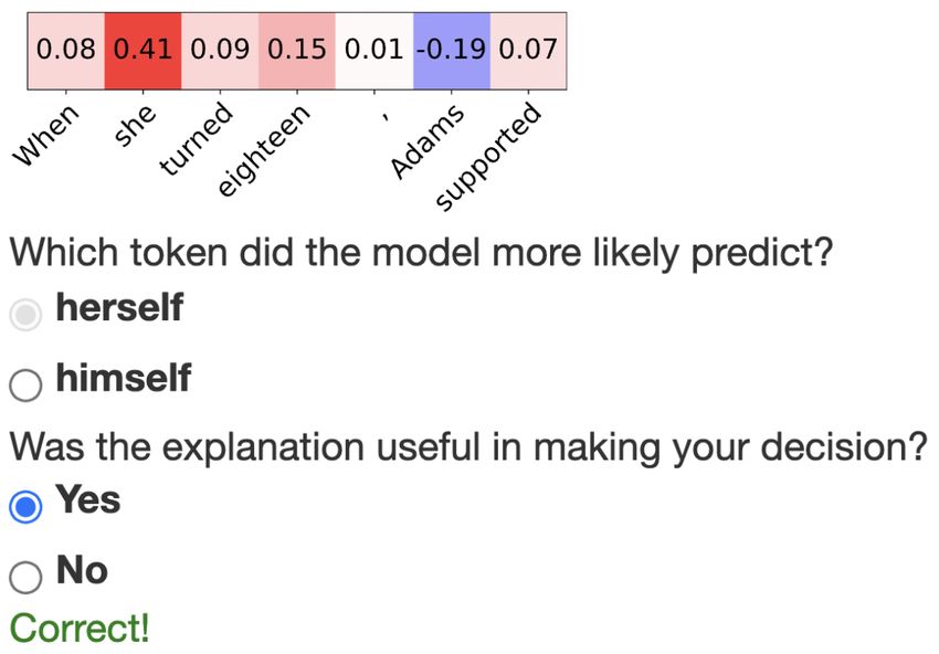
Figure 3: Example of a prompt in our human study. and Perktold, 2010) with the annotator and word pair as
random effects, the explanation method as fixed effect, and
the answer accuracy or usefulness as the dependent variable.
to distinguish from in our study (Appendix C). 10 of these In Appendix D we provide the results of the mixed-effects
word pairs were selected from the BLiMP dataset to reflect models we fitted.
a certain linguistic phenomenon, and the other 10 word
pairs were selected from pairs with the highest “confusion
Acc. Acc. Acc. Acc.
score” on the WikiText-103 test split (Merity et al., 2016). Acc. Correct Incorrect Useful Useful Not Useful
We define the confusion using the joint probability of a
None 61.38 74.50 48.25 – – –
confusion from token a to token b given a corpus X: SGI 64.00 78.25 49.75 62.12 67.20 58.75
∗
SGI 65.62 79.00 52.25 63.88 69.67 58.48
P (xtrue = a, xmodel = b) = SE 63.12 79.00 47.25 46.50 65.86 60.75
∗
1 X X SE 64.62 77.00 52.25 64.88 70.52 53.74
Pmodel (x̂t = b|xInterpreting Language Models with Contrastive Explanations
Phenomenon / Target Foil Cluster Embd Nearest Neighbors Example
POS
Anaphor he she, her, She, Her, herself, hers she,She, her, She, he, they, Her, we, it,she, That night , Ilsa confronts Rick in the de-
Agreement I, that,Her, you, was, there,He, is, as, in’ serted café . When he refuses to give her
the letters , _____
Animate man fruit, mouse, ship, acid, glass, water, tree, fruit, fruits, Fruit, meat, flower,fruit, You may not be surprised to learn that Kelly
Subject honey, sea, ice, smoke, wood, rock, sugar, tomato, vegetables, fish, apple, berries, Pool was neither invented by a _____
sand, cherry, dirt, fish, wind, snow food, citrus, banana, vegetable, strawberry,
fru, delicious, juice, foods
Determiner- page tabs, pages, icons, stops, boxes, doors, tabs, tab, Tab, apps, files, bags, tags, web- Immediately after "Heavy Competition"
Noun shortcuts, bags, flavours, locks, teeth, ears, sites, sections, browsers, browser, icons, first aired, NBC created a sub- _____
Agreement tastes, permissions, stairs, tickets, touches, buttons, pages, keeps, clips, updates, 28,
cages, saves, suburbs insists, 14
Subject-Verb go doesn, causes, looks, needs, makes, isn, doesn, isn, didn, does, hasn, wasn, don, Mala and the Eskimos _____
Agreement says, seems, seeks, displays, gives, wants, wouldn, makes, gets, has, is, aren, gives,
takes, uses, fav, contains, keeps, sees, tries, Doesn, couldn, seems, takes, keeps,doesn
sounds
ADJ black Black, white, black, White, red, BLACK, Black,Black, black,black, White, Although general relativity can be used to
green, brown, dark, orange, African, blue, BLACK, white, Blue, Red,White, In, perform a semi @-@ classical calculation
yellow, pink, purple, gray, grey, whites, B, The,The, It, red, Dark, 7, Green, of _____
Brown, silver African
ADJ black Asian, Chinese, English, Italian, American, Asian,Asian, Asia, Asians, Chinese, While taking part in the American Negro
Indian, East, South, British, Japanese, Euro- African, Japanese, Korean, China, Eu- Academy (ANA) in 1897 , Du Bois pre-
pean, African, Eastern, North, Washington, ropean, Indian, ethnic,Chinese, Japan, sented a paper in which he rejected Freder-
US, West, Australian, California, London American, Caucasian, Australian, His- ick Douglass ’s plea for _____
panic, white, Arab
ADP for to, in, and, on, with, for, when, from, at, (, if, to, in, for, on, and, as, with, of, a, at, that, The war of words would continue _____
as, after, by, over, because, while, without, the, from, by, an, (, To, is, it, or
before, through
ADV back the, to, a, in, and, on, of, it, ", not, that, with, the, a, an, it, this, that, in, The, to,The, all, One would have thought that claims dating
for, this, from, up, just, at, (, all and, their, as, for, on, his, at, some, what _____
DET his the, you, it, not, that, my, [, this, your, he, the, a, an, it, this, that, in, The, to,The, all, A preview screening of Sweet Smell of Suc-
all, so, what, there, her, some, his, time, and, their, as, for, on, his, at, some, what cess was poorly received , as Tony Cur-
him, He tis fans were expecting him to play one of
_____
NOUN girl Guy, Jack, Jones, Robin, James, David, Guy,Guy, guy,guy, Gu, Dave, Man, dude, Veronica talks to to Sean Friedrich and tells
Tom, Todd, Frank, Mike, Jimmy, Michael, Girl, Guys, John, Steve, \x00, \xef \xbf \xbd, him about the _____
Peter, George, William, Bill, Smith, Tony, \xef \xbf \xbd, \x1b, \xef \xbf \xbd, \x12,
Harry, Jackson \x1c, \x16
NUM five the, to, a, in, and, on, of, is, it, ", not, that, the, a, an, it, this, that, in, The, to,The, all, From the age of _____
1, with, for, 2, this, up, just, at and, their, as, for, on, his, at, some, what
VERB going got, didn, won, opened, told, went, heard, got, gets, get, had, went, gave, took, came, Truman had dreamed of _____
saw, wanted, lost, came, started, took, didn, did, getting, been, became, has, was,
gave, happened, tried, couldn, died, turned, made, started, have, gotten, showed
looked
Table 4: Examples of foil clusters obtained by clustering contrastive explanations of GPT-2. For each cluster, the 20 most
frequent foils are shown, as well as the 20 nearest neighbors in the word embedding space of the first foil, and an example is
included for the contrastive explanation of the target token vs. the underlined foil in the cluster. In each explanation, the two
most salient input tokens are highlighted in decreasing intensity of red.
6. What Context Do Models Use for Certain of a particular target word. Conceptually, this vector repre-
Decisions? sents the type of context that is necessary to disambiguate
the particular token from the target. Next, we use a cluster-
Finally, we use contrastive explanations to discover how ing algorithm on these vectors, generating clusters of foils
language models achieve various linguistic distinctions. We where similar types of context are useful to disambiguate.
hypothesize that similar evidence is necessary to disam- We then verify whether we find clusters associated with
biguate foils that are similar linguistically. To test this salient linguistic distinctions defined a-priori. Finally, we
hypothesis, we propose a methodology where we first rep- inspect the mean vectors of explanations associated with
resent each token by a vector representing its saliency map foils in the cluster to investigate how models perform these
when the token is used as a foil in contrastive explanation linguistic distinctions.Interpreting Language Models with Contrastive Explanations
6.1. Methodology inanimate nouns, the nearest neighbors of “fruit” are mostly
both singular and plural nouns related to produce.
We generate contrastive explanations for the 10 most fre-
quent words in each major part of speech as the target to- Plurality: For determiner-noun agreement, singular nouns
ken, and use the 10,000 most frequent vocabulary items are contrasted with clusters of plural noun foils, and vice-
as foils. For each target yt , we randomly select 500 versa. We find examples of clusters of plural nouns when the
sentences from the WikiText-103 dataset (Merity et al., target is a singular noun, whereas the nearest neighbors of
2016) and obtain a sentence set X. Then, for each foil “tabs” are both singular and plural nouns. To verify subject-
yf and each sentence xi ∈ X, we generate a single con- verb agreement, when the target is a plural verb, singular
trastive explanation e(xi , yt , yf ). Then, for each target yt verbs are clustered together, but the nearest neighbors of
and foil yf , L
we generate an aggregate explanation vector “doesn” contain both singular and plural verbs, especially
e(yt , yf ) = xi ∈X e(xi , yt , yf ) by concatenating the sin- negative contractions.
gle explanation vectors for each sentence in the corpus.
6.3. Explanation Analysis Results
Then, for a given target yt , we apply k-means clustering on
the concatenated contrastive explanations associated with By analyzing the explanations associated with different clus-
different foils yf to cluster foils by explanation similarity. ters, we are also able to learn various interesting properties
We use GPT-2 to extract all the contrastive explanations due of how GPT-2 makes certain predictions. We provide the
to its better alignment with linguistic phenomena than GPT- full results of our analysis in Appendix E.
Neo (§4). We only extract contrastive explanations with
gradient norm and gradient×input due to the computational For example, to distinguish between adjectives, the model
complexity of input erasure (§3.3). often relies on input words that are semantically similar to
the target: to distinguish “black” from other colors, words
In Table 4, we show examples of the obtained foil clusters. such as “relativity” are important. To contrast adpositions
The foils in each cluster are in descending frequency in and adverbs from other words with the same POS, verbs
training data. For the most frequent foil in each cluster, we in the input that are associated with the target word are
also retrieve its 20 nearest neighbors in the word embedding useful: for example, the verbs “dating” and “traced” are
space according to the Minkowski distance to compare them useful when the target is “back”.
with clusters of foils.
To choose the correct gender for determiners, nouns and
pronouns, the model often uses common proper nouns such
6.2. Foil Clusters
as “Veronica” and other gendered words such as “he” in the
First, we find that linguistically similar foils are indeed input. To disambiguate numbers from non-number words,
clustered together: we discover clusters relating to a variety input words related to enumeration or measurement (e.g.
of previously studied linguistic phenomena, a few of which “age”, “consists”, “least”) are useful. When the target word
we detail below and give examples in Table 4. Moreover, is a verb, other verbs in other verb forms are often clustered
foil clusters reflect linguistic distinctions that are not found together, which suggests that the model uses similar input
in the nearest neighbors of word embeddings. This suggests features to verify subject-verb agreement.
that the model use similar types of input features to make
Our analysis also reveals why the model may have made
certain decisions.
certain mistakes. For example, when the model generates
Anaphor agreement: To predict anaphor agreement, mod- a pronoun of the incorrect gender, often the model was
els must contrast pronouns from other pronouns with dif- influenced by a gender neutral proper noun in the input, or
ferent gender or number. We find that indeed, when the by proper nouns and pronouns of the opposite gender that
target is a pronoun, other pronouns of a different gender or appear in the input.
number are often clustered together: when the target is a
Overall, our methodology for clustering contrastive expla-
male pronoun, we find a cluster of female pronouns. The
nations provides an aggregate analysis of linguistic distinc-
foil cluster containing “she” includes several types of pro-
tions to understand general properties of language model
nouns that are all of the female gender. On the other hand,
decisions.
the nearest neighbors of “she” are mostly limited to subject
and object pronouns, and they are of various genders and
numbers. 7. Conclusion and Future Work
Animacy: In certain verb phrases, the main verb enforces In this work, we interpreted language model decisions us-
that the subject is animate. Reflecting this, when the target ing contrastive explanations by extending three existing
is an animate noun, inanimate nouns form a cluster. While input saliency methods to the contrastive setting. We also
the foil cluster in Table 4 contains a variety of singular proposed three new methods to evaluate and explore theInterpreting Language Models with Contrastive Explanations
quality of contrastive explanations: an alignment evaluation human? In Proceedings of the 2018 Conference on Em-
to verify whether explanations capture linguistically appro- pirical Methods in Natural Language Processing, pages
priate evidence, a user evaluation to measure the contrastive 1036–1042, Brussels, Belgium. Association for Compu-
model simulatability of explanations, and a clustering-based tational Linguistics.
aggregate analysis to investigate model properties using
contrastive explanations. Misha Denil, Alban Demiraj, and Nando De Freitas. 2014.
Extraction of salient sentences from labelled documents.
We find that contrastive explanations are better aligned to
arXiv preprint arXiv:1412.6815.
known evidence related to major grammatical phenomena
than their non-contrastive counterparts. Moreover, con- Finale Doshi-Velez and Been Kim. 2017. Towards a rig-
trastive explanations allow better contrastive simulatability orous science of interpretable machine learning. arXiv
of models for users. From there, we studied what kinds of preprint arXiv:1702.08608.
decisions require similar evidence and we used contrastive
explanations to characterize how models make certain lin- Leo Gao, Stella Biderman, Sid Black, Laurence Golding,
guistic distinctions. Overall, contrastive explanations give a Travis Hoppe, Charles Foster, Jason Phang, Horace He,
more intuitive and fine-grained interpretation of language Anish Thite, Noa Nabeshima, Shawn Presser, and Connor
models. Leahy. 2020. The Pile: An 800gb dataset of diverse text
Future work could explore the application of these con- for language modeling. arXiv preprint arXiv:2101.00027.
trastive explanations to other machine learning models and
tasks, extending other interpretability methods to the con- Peter Hase and Mohit Bansal. 2020. Evaluating explainable
trastive setting, as well as using what we learn about models AI: Which algorithmic explanations help users predict
through contrastive explanations to improve them. model behavior? In Proceedings of the 58th Annual
Meeting of the Association for Computational Linguistics,
pages 5540–5552, Online. Association for Computational
Acknowledgements Linguistics.
We would like to thank Danish Pruthi and Paul Michel for
initial discussions about this paper topic, Lucio Dery and Matthew Honnibal and Ines Montani. 2017. spaCy 2: Nat-
Patrick Fernandes for helpful feedback. We would also ural language understanding with Bloom embeddings,
like to thank Cathy Jiao, Clara Na, Chen Cui, Emmy Liu, convolutional neural networks and incremental parsing.
Karthik Ganesan, Kunal Dhawan, Shubham Phal, Sireesh To appear.
Gururaja and Sumanth Subramanya Rao for participating
Alon Jacovi, Swabha Swayamdipta, Shauli Ravfogel, Yanai
in the human evaluation. This work was supported by the
Elazar, Yejin Choi, and Yoav Goldberg. 2021. Contrastive
Siebel Scholars Award and the CMU-Portugal MAIA pro-
explanations for model interpretability. In Proceedings
gram.
of the 2021 Conference on Empirical Methods in Natu-
ral Language Processing, pages 1597–1611, Online and
References Punta Cana, Dominican Republic. Association for Com-
David Baehrens, Timon Schroeter, Stefan Harmeling, Mo- putational Linguistics.
toaki Kawanabe, Katja Hansen, and Klaus-Robert Müller.
Marcin Junczys-Dowmunt, Roman Grundkiewicz, Tomasz
2010. How to explain individual classification decisions.
Dwojak, Hieu Hoang, Kenneth Heafield, Tom Necker-
The Journal of Machine Learning Research, 11:1803–
mann, Frank Seide, Ulrich Germann, Alham Fikri Aji,
1831.
Nikolay Bogoychev, André F. T. Martins, and Alexandra
Yonatan Belinkov and James Glass. 2019. Analysis methods Birch. 2018. Marian: Fast neural machine translation in
in neural language processing: A survey. Transactions of C++. In Proceedings of ACL 2018, System Demonstra-
the Association for Computational Linguistics, 7:49–72. tions, pages 116–121, Melbourne, Australia. Association
for Computational Linguistics.
Sid Black, Leo Gao, Phil Wang, Connor Leahy, and Stella
Biderman. 2021. GPT-Neo: Large Scale Autoregressive Jiwei Li, Xinlei Chen, Eduard Hovy, and Dan Jurafsky.
Language Modeling with Mesh-Tensorflow. If you use 2016a. Visualizing and understanding neural models
this software, please cite it using these metadata. in NLP. In Proceedings of the 2016 Conference of the
North American Chapter of the Association for Computa-
Arjun Chandrasekaran, Viraj Prabhu, Deshraj Yadav, tional Linguistics: Human Language Technologies, pages
Prithvijit Chattopadhyay, and Devi Parikh. 2018. Do 681–691, San Diego, California. Association for Compu-
explanations make VQA models more predictable to a tational Linguistics.Interpreting Language Models with Contrastive Explanations
Jiwei Li, Will Monroe, and Dan Jurafsky. 2016b. Under- Eric Wallace, Jens Tuyls, Junlin Wang, Sanjay Subrama-
standing neural networks through representation erasure. nian, Matt Gardner, and Sameer Singh. 2019. AllenNLP
arXiv preprint arXiv:1612.08220. Interpret: A framework for explaining predictions of NLP
models. In Empirical Methods in Natural Language Pro-
Peter Lipton. 1990. Contrastive explanation. Royal Institute cessing.
of Philosophy Supplement, 27:247–266.
Alex Warstadt, Alicia Parrish, Haokun Liu, Anhad Mo-
Zachary C. Lipton. 2018. The mythos of model interpretabil- hananey, Wei Peng, Sheng-Fu Wang, and Samuel R. Bow-
ity: In machine learning, the concept of interpretability is man. 2020. BLiMP: The benchmark of linguistic minimal
both important and slippery. Queue, 16(3):31–57. pairs for English. Transactions of the Association for
Computational Linguistics, 8:377–392.
Andreas Madsen, Siva Reddy, and Sarath Chandar. 2021.
Post-hoc interpretability for neural nlp: A survey. arXiv Kayo Yin, Patrick Fernandes, André F. T. Martins, and
preprint arXiv:2108.04840. Graham Neubig. 2021a. When does translation require
context? a data-driven, multilingual exploration. arXiv
Ann L McGill and Jill G Klein. 1993. Contrastive and preprint arXiv:2109.07446.
counterfactual reasoning in causal judgment. Journal of
Kayo Yin, Patrick Fernandes, Danish Pruthi, Aditi Chaud-
Personality and Social Psychology, 64(6):897.
hary, André F. T. Martins, and Graham Neubig. 2021b.
Stephen Merity, Caiming Xiong, James Bradbury, and Do context-aware translation models pay the right atten-
Richard Socher. 2016. Pointer sentinel mixture models. tion? In Proceedings of the 59th Annual Meeting of the
arXiv preprint arXiv:1609.07843. Association for Computational Linguistics and the 11th
International Joint Conference on Natural Language Pro-
Danish Pruthi, Bhuwan Dhingra, Livio Baldini Soares, cessing (Volume 1: Long Papers), pages 788–801, Online.
Michael Collins, Zachary C Lipton, Graham Neubig, Association for Computational Linguistics.
and William W Cohen. 2020. Evaluating explanations:
Ruiqi Zhong, Steven Shao, and Kathleen R. McKeown.
How much do explanations from the teacher aid students?
2019. Fine-grained sentiment analysis with faithful atten-
arXiv preprint arXiv:2012.00893.
tion. CoRR, abs/1908.06870.
Alec Radford, Jeffrey Wu, Rewon Child, David Luan, Dario
Amodei, Ilya Sutskever, et al. 2019. Language models
are unsupervised multitask learners. OpenAI blog. A. Contrastive Explanations for Neural
Machine Translation (NMT) Models
Skipper Seabold and Josef Perktold. 2010. Statsmodels:
Econometric and statistical modeling with python. In A.1. Extending Contrastive Explanations to NMT
Proceedings of the 9th Python in Science Conference, Machine translation can be thought of as a specific type of
volume 57, page 61. Austin, TX. language models where the model is conditioned on both
the source sentence and the partial translation. It has similar
Avanti Shrikumar, Peyton Greenside, Anna Shcherbina, and
complexities as monolingual language modeling that make
Anshul Kundaje. 2016. Not just a black box: Learning
interpreting neural machine translation (NMT) models diffi-
important features through propagating activation differ-
cult. We therefore also extend contrastive explanations to
ences. arXiv preprint arXiv:1605.01713.
NMT models.
Karen Simonyan, Andrea Vedaldi, and Andrew Zisserman. We compute the contrastive gradient norm saliency for an
2013. Deep inside convolutional networks: Visualising NMT model by first calculating the gradient over the en-
image classification models and saliency maps. arXiv coder input (the source sentence) and over the decoder input
preprint arXiv:1312.6034. (the partial translation) as:
g ∗ (xei ) = ∇xei q(yt |xe , xd ) − q(yf |xe , xd )
Ilia Stepin, Jose M Alonso, Alejandro Catala, and Martín
Pereira-Fariña. 2021. A survey of contrastive and coun-
g ∗ (xdi ) = ∇xdi q(yt |xe , xd ) − q(yf |xe , xd )
terfactual explanation generation methods for explainable
artificial intelligence. IEEE Access, 9:11974–12001.
where xe is the encoder input, xd is the decoder input, and
Mukund Sundararajan, Ankur Taly, and Qiqi Yan. 2017. the other notations follow the ones in §3.1.
Axiomatic attribution for deep networks. In Interna-
Then, the contrastive gradient norm for each xei and xdi are:
tional Conference on Machine Learning, pages 3319–
∗
3328. PMLR. SGN (xei ) = ||g ∗ (xei )||L1Interpreting Language Models with Contrastive Explanations
∗
SGN (xdi ) = ||g ∗ (xdi )||L1 A.2. Qualitative Results
In Table 5, we provide examples of non-contrastive and
Similarly, the contrastive gradient × input are: contrastive explanations for NMT decisions. We use Mar-
∗
ianMT (Junczys-Dowmunt et al., 2018) with pre-trained
SGI (xei ) = g ∗ (xei ) · xei weights from the model trained to translate from English to
Romance languages5 to extract explanations. Each example
∗
SGI (xdi ) = g ∗ (xdi ) · xdi reflects a decision associated with one of the five types of
linguistic ambiguities during translation identified in Yin
We define the input erasure for each xei and xdi as: et al. (2021a).
∗ In the first example, the model must translate the gender
(xei ) = q(yt |xe , xd ) − q(yt |xe¬i , xd )
SE
neutral English pronoun “it” into the masculine French pro-
− q(yf |xe , xd ) − q(yf |xe¬i , xd )
noun “il”. In both non-contrastive and contrastive explana-
tions, the English antecedent “vase” influences the model
to predict “il”, however to disambiguate “il” from the fem-
∗
(xdi ) = q(yt |xe , xd ) − q(yt |xe , xd¬i )
SE inine pronoun “elle”, the model also relies on the french
antecedent and its masculine adjective “nouveau vase”.
− q(yf |xe , xd ) − q(yf |xe , xd¬i )
In the second example, the model must translate “your” with
the formality level consistent with the partial translation.
Why did the model predict "il" ? While in the non-contrastive explanation, only tokens in the
en: I ordered a new vase and it arrived today source sentence are salient which do not explain the model’s
fr: J ’ ai commandé un nouveau vase et choice of formality level, in the contrastive explanation,
Why did the model predict "il" instead of "elle" ? other French words in the polite formality level such as
en: I ordered a new vase and it arrived today
fr: J ’ ai commandé un nouveau vase et
“Vous” and “pouvez” are salient.
2. Why did the model predict "votre" ? In the third example, the model must translate “learned”
en: You cannot bring your dog here . using the verb form that is consistent with the partial transla-
fr: Vous ne pouvez pas amener tion. Similarly to the previous example, only the contrastive
Why did the model predict "votre" instead of "ton" ?
explanation contains salient tokens in the same verb from
en: You cannot bring your dog here .
fr: Vous ne pouvez pas amener as the target token such as “aimais”.
3. Why did the model predict "apprenais" ? In the fourth example, the model needs to resolve the elided
en: I liked school because I learned a lot there . verb in “I don’t know” to translate into French. The con-
fr: J ’ aimais l ’ école parce que j ’
trastive explanation with a different verb as a foil shows
Why did the model predict "apprenais" instead of "ai" ?
en: I liked school because I learned a lot there . that the elided verb in the target side makes the correct verb
fr: J ’ aimais l ’ école parce que j ’ more likely than another verb.
4. Why did the model predict "sais" ? In the fifth example, the model must choose the translation
en: They know what to do , I don ’ t . that is lexically cohesive with the partial translation, where
fr: Ils savent quoi faire , je ne
Why did the model predict "sais" instead of "veux" ? “carnet” refers to a book with paper pages and “ordinateur”
en: They know what to do , I don ’ t . refers to a computer notebook. In the non-contrastive expla-
fr: Ils savent quoi faire , je ne nation, the word “notebook” and the target token preceding
5. Why did the model predict "carnet" ? the prediction are the most salient. In the contrastive ex-
en: I like my old notebook better than my new notebook planation, the word “carnet” in the partial translation also
fr: J ’ aime mieux mon ancien carnet que mon nouveau becomes salient.
Why did the model predict "carnet" instead of "ordinateur" ?
en: I like my old notebook better than my new notebook
fr: J ’ aime mieux mon ancien carnet que mon nouveau B. Alignment of Contrastive Explanations to
Linguistic Paradigms
Table 5: Examples of non-contrastive and contrastive expla-
nations for NMT models translating from English to French In Table 6, we present the full alignment scores of con-
using input × gradient. Input tokens that are measured to trastive explanations from GPT-2 and GPT-Neo models with
raise or lower the probability of each decision are in red the known evidence to disambiguate linguistic paradigms in
and blue respectively, and those with little influence are in 5
https://github.com/Helsinki-NLP/Tatoeba-Challenge/blob/
white. master/models/eng-roa/README.mdInterpreting Language Models with Contrastive Explanations
the BLiMP dataset. Similarly to adpositions, LMs often use the verb associated
with the target adverb to contrast it from other adverbs. For
C. Highly Confusable Word Pairs example, the verbs “dating” and “traced” are useful when
the target is “back”, and the verbs “torn” and “lower” are
In Table 7, we provide the list of contrastive word pairs used useful when the target is “down”.
in our human study for model simulatability (§5). The first
10 pairs are taken from BLiMP linguistic paradigms and we Determiners. Other determiners are often clustered to-
provide the associated unique identifier for each pair. The gether when the target is a determiner. Particularly, when the
last 10 pairs are chosen from word pairs with the highest target is a possessive determiner, we find clusters with other
confusion score. possessive determiners, and when the target is a demonstra-
tive determiner, we find clusters with demonstrative deter-
D. Mixed Effects Models Results miners.
In Table 8, we show the results of fitting linear mixed-effects When the determiner is a gendered possessive determiner
models to the results of our user study for model simulata- such as “his”, proper nouns of the same gender, such as
bility (§5). “John” and “George”, are often useful. For demonstrative
determiners, such as “this”, verbs that are usually associated
with a targeted object, such as “achieve” and “angered” are
E. Analysis of Foil Clusters useful.
In Figure 4, we give a few examples of clusters and expla-
nations we obtain for each part of speech. For each part Nouns. When the target noun refers to a person, for exam-
of speech, we describe our findings in more detail in the ple, “girl”, foil nouns that also refer to a person form one
following. cluster (e.g. “woman”, “manager”, “friend”), commonly
male proper nouns form another (e.g. “Jack”, “Robin”,
“James”), commonly female proper nouns form another (e.g.
Adjectives. When the target word is an adjective, other “Sarah”, “Elizabeth”, “Susan”), and inanimate objects form
foil adjectives that are semantically similar to the target are a fourth (e.g. “window”, “fruit”, “box”).
often clustered together. For example, when the target is
“black”, we find one cluster with various color adjectives, When the target noun is an inanimate object, there are often
and we also find a different cluster with various adjectives two notable clusters: a cluster with singular inanimate nouns
relating to the race or nationality of a person. and a cluster with plural inanimate nouns. This suggests
how clustering foils by explanations confirm that certain
We find that to distinguish between different adjectives, grammatical phenomena require similar evidence for disam-
input words that are semantically close to the correct adjec- biguation; in this case, determiner-noun agreement.
tive are salient. For example to disambiguate the adjective
“black” from other colors, words such as “venom” and “rela- To predict a target animate noun such as “girl” instead
tivity” are important. of foil nouns that refer to a non-female or older person,
input words that are female names (e.g. “Meredith”) or that
refer to youth (e.g. “young”) are useful. To disambiguate
Adpositions. When the target is an adposition, other ad- from male proper nouns, input words that refer to female
positions are often in the same cluster. people (e.g. “Veronica”, “she”) or adjectives related to the
To distinguish between different adpositions, the verb as- target (e.g. “tall”) influence the model to generate a female
sociated with the adposition is often useful to the LM. For common noun. To disambiguate from female proper nouns,
example, when the target word is “from”, verbs such as adjectives and determiners are useful. To disambiguate from
“garnered” and “released” helps the model distinguish the inanimate objects, words that describe a human or a human
target from other adpositions that are less commonly paired action (e.g. “delegate”, “invented”) are useful.
with these verbs (e.g. “for”, “of”). As another example, To predict a target inanimate noun such as “page” instead
for the target word “for”, verbs that indicate a long-lasting of nouns that are also singular, input words with similar
action such as “continue” and “lived” help the model dis- semantics are important such as “sheet” and “clicking” are
ambiguate. important. For plural noun foils, the determiner (e.g. “a”) is
important.
Adverbs. When the target is an adverb, other adverbs are
often clustered together. Sometimes, when the target is a Numbers. When the target is a number, non-number
specific type of adverb, such as an adverb of place, we can words often form one cluster and other numbers form an-
find a cluster with other adverbs of the same type. other cluster.Interpreting Language Models with Contrastive Explanations
GPT-2 GPT-Neo
Paradigm Dist Explanation Dot Product (↑) Probes Needed (↓) MRR (↑) Dot Product (↑) Probes Needed (↓) MRR (↑)
Random 0.528 0.706 0.718 0.548 0.618 0.762
SGN 0.429 1.384 0.478 0.480 0.828 0.622
∗
SGN 0.834 0.472 0.809 0.785 0.432 0.815
anaphor_gender_agreement 2.94 SGI 0.078 1.402 0.468 -0.054 0.526 0.786
∗
SGI -0.019 0.502 0.791 -0.133 0.684 0.747
SE -0.350 0.564 0.764 0.645 0.078 0.963
∗
SE 0.603 0.090 0.964 0.637 0.156 0.903
Random 0.554 0.666 0.741 0.568 0.598 0.756
SGN 0.463 1.268 0.512 0.508 0.784 0.639
∗
SGN 0.841 0.702 0.677 0.816 0.524 0.763
anaphor_number_agreement 2.90 SGI 0.084 1.346 0.497 -0.095 0.510 0.797
∗
SGI 0.084 0.408 0.860 -0.068 0.636 0.775
SE -0.349 0.704 0.728 0.618 0.128 0.940
∗
SE 0.604 0.136 0.951 0.666 0.106 0.956
Random 0.155 2.940 0.378 0.150 2.976 0.379
SGN 0.211 1.080 0.699 0.236 0.828 0.727
∗
SGN 0.463 0.754 0.749 0.452 0.862 0.721
animate_subject_passive 3.27 SGI 0.016 4.004 0.233 0.020 2.780 0.416
∗
SGI 0.069 2.782 0.412 0.016 2.844 0.409
SE -0.036 3.214 0.362 0.168 2.024 0.444
∗
SE 0.125 2.122 0.500 0.123 2.120 0.517
Random 0.208 2.202 0.449 0.207 2.142 0.461
SGN 0.239 1.320 0.598 0.150 2.954 0.287
∗
SGN 0.275 2.680 0.406 0.258 2.906 0.302
determiner_noun_agreement_1 1.00 SGI 0.560 0.038 0.983 -0.042 2.384 0.380
∗
SGI 0.162 1.558 0.603 -0.056 2.554 0.371
SE 0.022 1.150 0.604 0.234 1.290 0.543
∗
SE 0.031 2.598 0.363 0.362 0.612 0.811
Random 0.198 2.248 0.437 0.202 2.110 0.456
SGN 0.236 1.228 0.616 0.160 2.716 0.324
∗
SGN 0.286 2.578 0.380 0.266 2.826 0.310
determiner_noun_agreement_irregular_1 1.00 SGI 0.559 0.034 0.984 -0.035 2.160 0.419
∗
SGI 0.046 2.038 0.507 -0.046 2.428 0.374
SE 0.020 1.082 0.628 0.205 1.360 0.548
∗
SE 0.026 2.502 0.352 0.306 0.784 0.755
Random 0.167 2.672 0.406 0.168 2.672 0.405
SGN 0.118 3.914 0.237 0.120 3.902 0.230
∗
SGN 0.210 3.532 0.267 0.228 3.814 0.245
determiner_noun_agreement_with_adjective_1 2.05 SGI 0.118 2.426 0.354 -0.010 2.736 0.356
∗
SGI 0.141 2.012 0.482 -0.051 2.950 0.342
SE 0.042 1.730 0.583 0.092 2.748 0.333
∗
SE 0.305 1.084 0.680 0.260 1.176 0.697
Random 0.167 2.620 0.401 0.158 2.820 0.392
SGN 0.116 3.920 0.240 0.125 3.620 0.248
∗
SGN 0.205 3.664 0.256 0.228 3.718 0.243
determiner_noun_agreement_with_adj_irregular_1 2.07 SGI 0.106 2.620 0.345 -0.007 2.754 0.358
∗
SGI 0.111 2.244 0.448 -0.047 3.126 0.316
SE 0.048 1.688 0.586 0.103 2.644 0.347
∗
SE 0.313 1.024 0.686 0.263 1.066 0.683
Random 0.336 1.080 0.604 0.350 0.984 0.632
SGN 0.294 1.160 0.510 0.376 0.454 0.778
∗
SGN 0.456 0.450 0.787 0.449 0.382 0.812
npi_present_1 3.19 SGI 0.100 1.374 0.463 -0.160 1.288 0.575
∗
SGI 0.144 0.570 0.759 0.202 0.766 0.752
SE -0.336 1.514 0.556 0.624 0.086 0.960
∗
SE 0.160 0.902 0.684 0.062 1.204 0.556
Random 0.230 1.936 0.494 0.227 2.106 0.463
SGN 0.266 1.199 0.584 0.269 0.965 0.646
∗
SGN 0.408 1.092 0.619 0.392 1.000 0.649
distractor_agreement_relational_noun 3.94 SGI 0.044 2.291 0.369 -0.066 2.326 0.434
∗
SGI 0.223 1.057 0.631 0.051 1.383 0.591
SE -0.023 1.922 0.434 0.120 2.007 0.400
∗
SE 0.190 1.709 0.502 0.186 1.617 0.544
Random 0.561 0.539 0.760 0.545 0.494 0.769
SGN 0.652 0.242 0.917 0.610 0.348 0.860
∗
SGN 0.676 0.315 0.843 0.644 0.376 0.817
irregular_plural_subject_verb_agreement_1 1.11 SGI 0.590 0.253 0.912 0.067 0.472 0.783
∗
SGI 0.348 0.298 0.864 0.021 0.489 0.750
SE -0.570 0.787 0.617 -0.021 0.893 0.553
∗
SE 0.264 0.635 0.673 0.267 0.584 0.734
Random 0.694 0.316 0.853 0.693 0.336 0.849
SGN 0.740 0.194 0.946 0.724 0.268 0.906
∗
SGN 0.756 0.251 0.909 0.747 0.274 0.898
regular_plural_subject_verb_agreement_1 1.13 SGI 0.748 0.202 0.944 -0.039 0.333 0.852
∗
SGI 0.371 0.242 0.889 0.039 0.262 0.879
SE -0.614 0.610 0.718 0.303 0.632 0.694
∗
SE 0.584 0.353 0.836 0.568 0.313 0.842
Table 6: Alignment of GPT-2 and GPT-Neo explanations with BLiMP. Scores better than their (non-)contrastive counterparts
are bolded. “Dist” gives the average distance from the target to the important context token.You can also read