Image Super-Resolution via Iterative Refinement
←
→
Page content transcription
If your browser does not render page correctly, please read the page content below

Image Super-Resolution via Iterative Refinement

                                           Chitwan Saharia†, Jonathan Ho, William Chan, Tim Salimans, David J. Fleet, Mohammad Norouzi
                                       {sahariac,jonathanho,williamchan,salimans,davidfleet,mnorouzi}@google.com
                                                                                                 Google Research, Brain Team
arXiv:2104.07636v2 [eess.IV] 30 Jun 2021

                                                                        Abstract                                     Input             SR3 output           Reference

                                               We present SR3, an approach to image Super-Resolution
                                           via Repeated Refinement. SR3 adapts denoising diffusion
                                           probabilistic models [17, 48] to conditional image gener-
                                           ation and performs super-resolution through a stochastic
                                           iterative denoising process. Output generation starts with
                                           pure Gaussian noise and iteratively refines the noisy output
                                           using a U-Net model trained on denoising at various noise
                                           levels. SR3 exhibits strong performance on super-resolution
                                           tasks at different magnification factors, on faces and natu-
                                           ral images. We conduct human evaluation on a standard
                                           8× face super-resolution task on CelebA-HQ, comparing
                                           with SOTA GAN methods. SR3 achieves a fool rate close
                                           to 50%, suggesting photo-realistic outputs, while GANs do
                                                                                                              Figure 1: Two representative SR3 outputs: (top) 8× face super-
                                           not exceed a fool rate of 34%. We further show the effec-
                                                                                                              resolution at 16×16→128×128 pixels (bottom) 4× natural image
                                           tiveness of SR3 in cascaded image generation, where gen-
                                                                                                              super-resolution at 64×64→256×256 pixels.
                                           erative models are chained with super-resolution models,
                                           yielding a competitive FID score of 11.3 on ImageNet.
                                                                                                              GANs [14, 19, 36] have shown convincing image genera-
                                           1. Introduction                                                    tion results and have been applied to conditional tasks such
                                                                                                              as image super-resolution [7, 8, 25, 28, 33]. However, these
                                              Single-image super-resolution is the process of generat-        approaches often suffer from various limitations; e.g., au-
                                           ing a high-resolution image that is consistent with an in-         toregressive models are prohibitively expensive for high-
                                           put low-resolution image. It falls under the broad family          resolution image generation, NFs and VAEs often yield
                                           of image-to-image translation tasks, including colorization,       sub-optimal sample quality, and GANs require carefully de-
                                           in-painting, and de-blurring. Like many such inverse prob-         signed regularization and optimization tricks to tame opti-
                                           lems, image super-resolution is challenging because multi-         mization instability [2, 15] and mode collapse [29, 38].
                                           ple output images may be consistent with a single input im-
                                                                                                                  We propose SR3 (Super-Resolution via Repeated Re-
                                           age, and the conditional distribution of output images given
                                                                                                              finement), a new approach to conditional image generation,
                                           the input typically does not conform well to simple para-
                                                                                                              inspired by recent work on Denoising Diffusion Probabilis-
                                           metric distributions, e.g., a multivariate Gaussian. Accord-
                                                                                                              tic Models (DDPM) [17, 47], and denoising score match-
                                           ingly, while simple regression-based methods with feedfor-
                                                                                                              ing [17, 49]. SR3 works by learning to transform a stan-
                                           ward convolutional nets may work for super-resolution at
                                                                                                              dard normal distribution into an empirical data distribu-
                                           low magnification ratios, they often lack the high-fidelity
                                                                                                              tion through a sequence of refinement steps, resembling
                                           details needed for high magnification ratios.
                                                                                                              Langevin dynamics. The key is a U-Net architecture [42]
                                              Deep generative models have seen success in learning
                                                                                                              that is trained with a denoising objective to iteratively re-
                                           complex empirical distributions of images (e.g., [52, 57]).
                                                                                                              move various levels of noise from the output. We adapt
                                           Autoregressive models [31, 32], variational autoencoders
                                                                                                              DDPMs to conditional image generation by proposing a
                                           (VAEs) [24, 54], Normalizing Flows (NFs) [10, 23], and
                                                                                                              simple and effective modification to the U-Net architecture.
                                             † Work   done as part of the Google AI Residency.                In contrast to GANs that require inner-loop maximization,
we minimize a well-defined loss function. Unlike autore-        y0 ∼ p(y | x)     yt−1                        yt     yT ∼ N (0, I)
gressive models, SR3 uses a constant number of inference                                    q(yt |yt−1 )
steps regardless of output resolution.
    SR3 works well across a range of magnification factors                                pθ (yt−1 |yt , x)
and input resolutions. SR3 models can also be cascaded,
e.g., going from 64×64 to 256×256, and then to 1024×1024.       Figure 2: The forward diffusion process q (left to right) gradually
Cascading models allows one to independently train a few        adds Gaussian noise to the target image. The reverse inference
small models rather than a single large model with a high       process p (right to left) iteratively denoises the target image con-
                                                                ditioned on a source image x. Source image x is not shown here.
magnification factor. We find that chained models enable
more efficient inference, since directly generating a high-
resolution image requires more iterative refinement steps       be consistent with a single source image. We are interested
for the same quality. We also find that one can chain an un-    in learning a parametric approximation to p(y | x) through
conditional generative model with SR3 models to uncondi-        a stochastic iterative refinement process that maps a source
tionally generate high-fidelity images. Unlike existing work    image x to a target image y ∈ Rd . We approach this
that focuses on specific domains (e.g., faces), we show that    problem by adapting the denoising diffusion probabilistic
SR3 is effective on both faces and natural images.              (DDPM) model of [17, 47] to conditional image generation.
    Automated image quality scores like PSNR and SSIM               The conditional DDPM model generates a target im-
do not reflect human preference well when the input reso-       age y0 in T refinement steps. Starting with a pure noise
lution is low and the magnification ratio is large (e.g., [3,   image yT ∼ N (0, I), the model iteratively refines the
7, 8, 28]). These quality scores often penalize synthetic       image through successive iterations (yT −1 , yT −2 , . . . , y0 )
high-frequency details, such as hair texture, because syn-      according to learned conditional transition distributions
thetic details do not perfectly align with the reference de-    pθ (yt−1 | yt , x) such that y0 ∼ p(y | x) (see Figure 2).
tails. We resort to human evaluation to compare the qual-           The distributions of intermediate images in the inference
ity of super-resolution methods. We adopt a 2-alternative       chain are defined in terms of a forward diffusion process
forced-choice (2AFC) paradigm in which human subjects           that gradually adds Gaussian noise to the signal via a fixed
are shown a low-resolution input and are required to select     Markov chain, denoted q(yt | yt−1 ). The goal of our model
between a model output and a ground truth image (cf. [63]).     is to reverse the Gaussian diffusion process by iteratively re-
Based on this study, we calculate fool rate scores that cap-    covering signal from noise through a reverse Markov chain
ture both image quality and the consistency of model out-       conditioned on x. In principle, each forward process step
puts with low-resolution inputs. Experiments demonstrate        can be conditioned on x too, but we leave that to future
that SR3 achieves a significantly higher fool rate than SOTA    work. We learn the reverse chain using a neural denoising
GAN methods [7, 28] and a strong regression baseline.           model fθ that takes as input a source image and a noisy tar-
                                                                get image and estimates the noise. We first give an overview
Our key contributions are summarized as:
                                                                of the forward diffusion process, and then discuss how our
 • We adapt denoising diffusion models to conditional im-
                                                                denoising model fθ is trained and used for inference.
   age generation. Our method, SR3, is an approach to im-
   age super-resolution via iterative refinement.               2.1. Gaussian Diffusion Process
 • SR3 proves effective on face and natural image super-
                                                                   Following [17, 47], we first define a forward Markovian
   resolution at different magnification factors. On a stan-
                                                                diffusion process q that gradually adds Gaussian noise to a
   dard 8× face super-resolution task, SR3 achieves a hu-
                                                                high-resolution image y0 over T iterations:
   man fool rate close to 50%, outperforming FSRGAN [7]
   and PULSE [28] that achieve fool rates of at most 34%.                               YT
                                                                     q(y1:T | y0 ) =            q(yt | yt−1 ) ,         (1)
 • We demonstrate unconditional and class-conditional gen-                                  t=1
                                                                                                 √
   eration by cascading a 64×64 image synthesis model with           q(yt | yt−1 ) = N (yt | αt yt−1 , (1 − αt )I) , (2)
   SR3 models to progressively generate 1024×1024 uncon-
                                                                where the scalar parameters α1:T are hyper-parameters,
   ditional faces in 3 stages, and 256×256 class-conditional
                                                                subject to 0 < αt < 1, which determine the variance of the
   ImageNet samples in 2 stages. Our class conditional Im-
                                                                noise added at each iteration. Note that yt−1 is attenuated
   ageNet samples attain competitive FID scores.                   √
                                                                by αt to ensure that the variance of the random variables
2. Conditional Denoising Diffusion Model                        remains bounded as t → ∞. For instance, if the variance of
                                                                yt−1 is 1, then the variance of yt is also 1.
   We are given a dataset of input-output image pairs, de-         Importantly, one can characterize the distribution of yt
noted D = {xi , yi }N
                    i=1 , which represent samples drawn         given y0 by marginalizing out the intermediate steps as
from an unknown conditional distribution p(y | x). This is
                                                                                                √
a one-to-many mapping in which many target images may                   q(yt | y0 ) = N (yt | γt y0 , (1 − γt )I) ,     (3)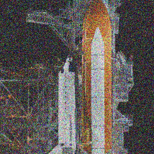
Algorithm 1 Training a denoising model fθ                          Algorithm 2 Inference in T iterative refinement steps
 1: repeat                                                          1: yT ∼ N (0, I)
 2: (x, y0 ) ∼ p(x, y)                                              2: for t = T, . . . , 1 do
 3: γ ∼ p(γ)                                                        3: z ∼ N (0, I)     if t > 1, else z = 0
 4:  ∼ N (0, I)                                                                               1−αt
                                                                                                                              √
                                                                    4:  yt−1 = √1αt yt −       √    f (x, yt , γt )
                                                                                                1−γt θ
                                                                                                                           +    1 − αt z
 5: Take a gradient descent step on
                      √     √                 p                     5: end for
         ∇θ fθ (x,     γy0 + 1 − γ, γ) −    p
 6: until converged                                                 6: return y0

               Qt
where γt = i=1 αi . Furthermore, with some algebraic               values of  and y0 can be derived from each other determin-
manipulation and completing the square, one can derive the         istically, but changing the regression target has an impact on
posterior distribution of yt−1 given (y0 , yt ) as                 the scale of the loss function. We expect both of these vari-
                                                                   ants to work reasonably well if p(γ) is modified to account
      q(yt−1 | y0 , yt ) = N (yt−1 | µ, σ 2 I)                     for the scale of the loss function. Further investigation of
            √                      √
              γt−1 (1 − αt )         αt (1 − γt−1 )                the loss function used for training the denoising model is an
       µ=                     y0 +                  yt       (4)
                 1 − γt                 1 − γt                     interesting avenue for future research in this area.
             (1 − γt−1 )(1 − αt )
       σ2 =                        .                               2.3. Inference via Iterative Refinement
                     1 − γt
                                                                      Inference under our model is defined as a reverse Marko-
This posterior distribution is helpful when parameterizing
                                                                   vian process, which goes in the reverse direction of the for-
the reverse chain and formulating a variational lower bound
                                                                   ward diffusion process, starting from Gaussian noise yT :
on the log-likelihood of the reverse chain. We next discuss
how one can learn a neural network to reverse this Gaussian                                             YT
diffusion process.                                                           pθ (y0:T |x)    = p(yT )               pθ (yt−1 |yt , x) (7)
                                                                                                            t=1
                                                                                  p(yT )     = N (yT | 0, I)                                (8)
2.2. Optimizing the Denoising Model
                                                                         pθ (yt−1 |yt , x)   = N (yt−1 |        µθ (x, yt , γt ), σt2 I)   . (9)
   To help reverse the diffusion process, we take advantage
of additional side information in the form of a source image       We define the inference process in terms of isotropic Gaus-
x and optimize a neural denoising model fθ that takes as           sian conditional distributions, pθ (yt−1 |yt , x), which are
input this source image x and a noisy target image ye,             learned. If the noise variance of the forward process steps
             √         p                                           are set as small as possible, i.e., α1:T ≈ 1, the optimal re-
        ye = γ y0 + 1 − γ  ,           ∼ N (0, I) ,    (5)       verse process p(yt−1 |yt , x) will be approximately Gaus-
and aims to recover the noiseless target image y0 . This           sian [47]. Accordingly, our choice of Gaussian conditionals
definition of a noisy target image ye is compatible with the       in the inference process (9) can provide a reasonable fit to
marginal distribution of noisy images at different steps of        the true reverse process. Meanwhile, 1 − γT should be large
the forward diffusion process in (3).                              enough so that yT is approximately distributed according
    In addition to a source image x and a noisy target im-         to the prior p(yT ) = N (yT |0, I), allowing the sampling
age ye, the denoising model fθ (x, ye, γ) takes as input the       process to start at pure Gaussian noise.
sufficient statistics for the variance of the noise γ, and is         Recall that the denoising model fθ is trained to estimate
trained to predict the noise vector . We make the denois-         , given any noisy image ye including yt . Thus, given yt ,
ing model aware of the level of noise through conditioning         we approximate y0 by rearranging the terms in (5) as
on a scalar γ, similar to [49, 6]. The proposed objective                         1      p
function for training fθ is                                                ŷ0 = √    yt − 1 − γt fθ (x, yt , γt ) .                       (10)
                                                                                   γt
                                                     p
                     √       p
   E(x,y) E,γ fθ (x, γ y0 + 1 − γ , γ) −              ,   (6)   Following the formulation of [17], we substitute our esti-
                                                     p
                                                                   mate ŷ0 into the posterior distribution of q(yt−1 |y0 , yt ) in
                     |      {z     }
                                y
                                e
                                                                   (4) to parameterize the mean of pθ (yt−1 |yt , x) as
where  ∼ N (0, I), (x, y) is sampled from the training
dataset, p ∈ {1, 2}, and γ ∼ p(γ). The distribution of γ has                             1            1 − αt
                                                                     µθ (x, yt , γt ) = √      yt − √         fθ (x, yt , γt ) ,
a big impact on the quality of the model and the generated                                αt           1 − γt
outputs. We discuss our choice of p(γ) in Section 2.4.                                                                         (11)
   Instead of regressing the output of fθ to , as in (6), one     and we set the variance of pθ (yt−1 |yt , x) to (1 − αt ), a
can also regress the output of fθ to y0 . Given γ and ye, the      default given by the variance of the forward process [17].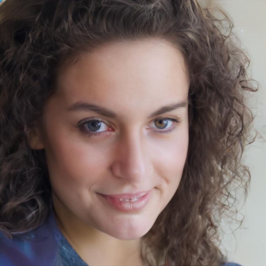
Following this parameterization, each iteration of itera-      els is expensive, limiting application to low-resolution im-
tive refinement under our model takes the form,                   ages. Normalizing flows [40, 10, 23] improve on sampling
                                                                  speed while modelling the exact data likelihood, but the
                                                 √

           1           1 − αt                                     need for invertible parameterized transformations with a
yt−1 ← √         yt − √        fθ (x, yt , γt ) + 1 − αt t ,
            αt          1 − γt                                    tractable Jacobian determinant limits their expressiveness.
                                                                  VAEs [24, 41] offer fast sampling, but tend to underper-
where t ∼ N (0, I). This resembles one step of Langevin          form GANs and ARs in image quality [54]. Generative
dynamics with fθ providing an estimate of the gradient of         Adversarial Networks (GANs) [14] are popular for class
the data log-density. We justify the choice of the training       conditional image generation and super-resolution. Nev-
objective in (6) for the probabilistic model outlined in (9)      ertheless, the inner-outer loop optimization often requires
from a variational lower bound perspective and a denoising        tricks to stabilize training [2, 15], and conditional tasks like
score-matching perspective in Appendix B.                         super-resolution usually require an auxiliary consistency-
2.4. SR3 Model Architecture and Noise Schedule                    based loss to avoid mode collapse [25]. Cascades of GAN
                                                                  models have been used to generate higher resolution images
   The SR3 architecture is similar to the U-Net found in          [9].
DDPM [17], with modifications adapted from [51]; we                   Score matching [18] models the gradient of the data log-
replace the original DDPM residual blocks with residual           density with respect to the image. Score matching on noisy
blocks from BigGAN [4], and we re-scale skip connections          data, called denoising score matching [58], is equivalent
by √12 . We also increase the number of residual blocks,          to training a denoising autoencoder, and to DDPMs [17].
and the channel multipliers at different resolutions (see Ap-     Denoising score matching over multiple noise scales with
pendix A for details). To condition the model on the in-          Langevin dynamics sampling from the learned score func-
put x, we up-sample the low-resolution image to the target        tions has recently been shown to be effective for high qual-
resolution using bicubic interpolation. The result is con-        ity unconditional image generation [49, 17]. These models
catenated with yt along the channel dimension. We exper-          have also been generalized to continuous time [51]. Denois-
imented with more sophisticated methods of conditioning,          ing score matching and diffusion models have also found
such as using FiLM [34], but we found that the simple con-        success in shape generation [5], and speech synthesis [6].
catenation yielded similar generation quality.                    We extend this method to super-resolution, with a simple
   For our training noise schedule, weP  follow [6], and use a    learning objective, a constant number of inference genera-
                                           T
piece wise distribution for γ, p(γ) = t=1 T1 U (γt−1 , γt ).      tion steps, and high quality generation.
Specifically, during training, we first uniformly sample
                                                                  Super-Resolution. Numerous super-resolution methods
a time step t ∼ {0, ..., T } followed by sampling γ ∼
                                                                  have been proposed in the computer vision community
U (γt−1 , γt ). We set T = 2000 in all our experiments.
                                                                  [11, 1, 22, 53, 25, 44]. Much of the early work on super-
   Prior work of diffusion models [17, 51] require 1-2k dif-
                                                                  resolution is regression based and trained with an MSE loss
fusion steps during inference, making generation slow for
                                                                  [11, 1, 60, 12, 21]. As such, they effectively estimate the
large target resolution tasks. We adapt techniques from [6]
                                                                  posterior mean, yielding blurry images when the posterior
to enable more efficient inference. Our model conditions
                                                                  is multi-modal [25, 44, 28]. Our regression baseline defined
on γ directly (vs t as in [17]), which allows us flexibility in
                                                                  below is also a one-step regression model trained with MSE
choosing number of diffusion steps, and the noise schedule
                                                                  (cf. [1, 21]), but with a large U-Net architecture. SR3, by
during inference. This has been demonstrated to work well
                                                                  comparison, relies on a series of iterative refinement steps,
for speech synthesis [6], but has not been explored for im-
                                                                  each of which is trained with a regression loss. This differ-
ages. For efficient inference we set the maximum inference
                                                                  ence permits our iterative approach to capture richer distri-
budget to 100 diffusion steps, and hyper-parameter search
                                                                  butions. Further, rather than estimating the posterior mean,
over the inference noise schedule. This search is inexpen-
                                                                  SR3 generates samples from the target posterior.
sive as we only need to train the model once [6]. We use
                                                                     Autoregressive models have been used successfully for
FID on held out data to choose the best noise schedule, as
                                                                  super-resolution and cascaded up-sampling [8, 27, 56, 33].
we found PSNR did not correlate well with image quality.
                                                                  Nevertheless, the expensive of inference limits their appli-
                                                                  cability to low-resolution images. SR3 can generate high-
3. Related Work
                                                                  resolution images, e.g., 1024×1024, but with a constant
SR3 is inspired by recent work on deep generative models          number of refinement steps (often no more than 100).
and recent learning-based approaches to super-resolution.            Normalizing flows have been used for super-resolution
Generative Models. Autoregressive models (ARs) [55, 45]           with a multi-scale approach [62]. They are capable of gen-
can model exact data log likelihood, capturing rich dis-          erating 1024×1024 images due in part to their efficient in-
tributions. However, their sequential generation of pix-          ference process. But SR3 uses a series of reverse diffusion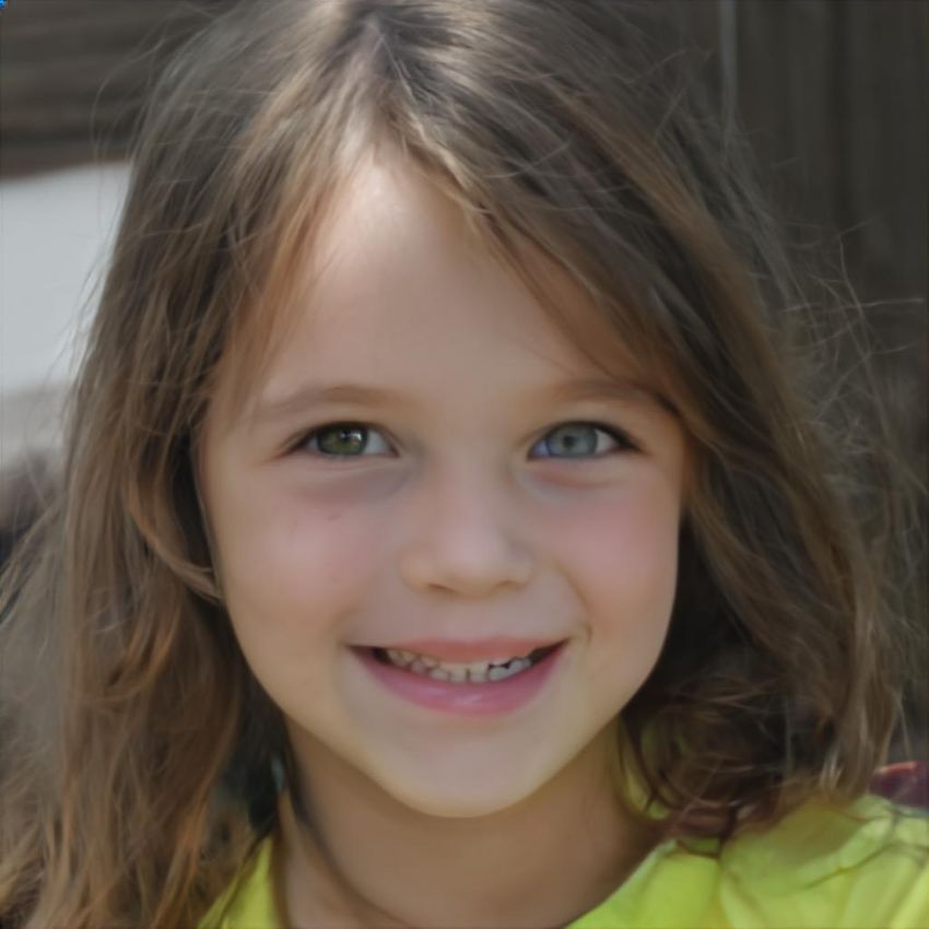
Bicubic                      Regression      SR3 (ours)              Reference

Figure 3: Results of a SR3 model (64×64 → 256×256), trained on ImageNet and evaluated on two ImageNet test images. For each we
also show an enlarged patch in which finer details are more apparent. Additional samples are shown in Appendix C.3 and C.4.

steps to transform a Gaussian distribution to an image dis-             baseline model that shares the same architecture as SR3, but
tribution while flows require a deep and invertible network.            is trained with a MSE loss. Our experiments include:
    GAN-based super-resolution methods have also found                   • Face super-resolution at 16×16 → 128×128 and 64×64 →
considerable success [19, 25, 28, 61, 44]. FSRGAN [7] and                  512 × 1512 trained on FFHQ and evaluated on CelebA-
PULSE [28] in particular have demonstrated high quality                    HQ.
face super-resolution results. However, many such GAN                    • Natural image super-resolution at 64 × 64 → 256 × 256
based methods are generally difficult to optimize, and often               pixels on ImageNet [43].
require auxiliary objective functions to ensure consistency
                                                                         • Unconditional 1024×1024 face generation by a cascade
with the low resolution inputs.
                                                                           of 3 models, and class-conditional 256 × 256 ImageNet
                                                                           image generation by a cascade of 2 models.
4. Experiments
                                                                        Datasets: We follow previous work [28], training face
   We assess the effectiveness of SR3 models in super-
                                                                        super-resolution models on Flickr-Faces-HQ (FFHQ) [20]
resolution on faces, natural images, and synthetic images
                                                                        and evaluating on CelebA-HQ [19]. For natural image
obtained from a low-resolution generative model. The latter
                                                                        super-resolution, we train on ImageNet 1K [43] and use
enables high-resolution image synthesis using model cas-
                                                                        the dev split for evaluation. We train unconditional face
cades. We compare SR3 with recent methods such as FSR-
                                                                        and class-conditional ImageNet generative models using
GAN [7] and PULSE [28] using human evaluation1 , and re-
                                                                        DDPM on the same datasets discussed above. For training
port FID for various tasks. We also compare to a regression
                                                                        and testing, we use low-resolution images that are down-
  1 Samples   generously provided by the authors of [28]                sampled using bicubic interpolation with anti-aliasing en-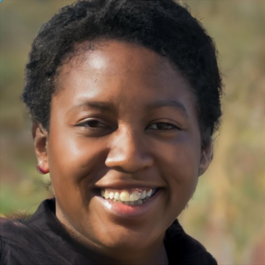
Bicubic                Regression               SR3 (ours)               Reference

Figure 4: Results of a SR3 model (64×64 → 512×512), trained on FFHQ, and applied to images outside of the training set, along with
enlarged patches to show finer details. Additional results are shown in Appendix C.1 and C.2.

abled. For ImageNet, we discard images where the shorter           (See Appendix A for task specific architectural details.)
side is less than the target resolution. We use the largest
central crop like [4], which is then resized to the target res-    4.1. Qualitative Results
olution using area resampling as our high resolution image.
                                                                       Natural Images: Figure 3 gives examples of super-
Training Details: We train all of our SR3 and regression           resolution natural images for 64×64 → 256×256 on the
models for 1M training steps with a batch size of 256. We          ImageNet dev set, along with enlarged patches for finer in-
choose a checkpoint for the regression baseline based on           spection. The baseline Regression model generates images
peak-PSNR on the held out set. We do not perform any               that are faithful to the inputs, but are blurry and lack detail.
checkpoint selection on SR3 models and simply select the           By comparison, SR3 produces sharp images with more de-
latest checkpoint. Consistent with [17], we use the Adam           tail; this is most evident in the enlarged patches. For more
optimizer with a linear warmup schedule over 10k train-            samples see Appendix C.3 and C.4.
ing steps, followed by a fixed learning rate of 1e-4 for SR3           Face Images: Figure 4 shows outputs of a face super-
models and 1e-5 for regression models. We use 625M pa-             resolution model (64×64 → 512×512) on two test images,
rameters for our 64 × 64 → {256 × 256, 512 × 512} mod-             again with selected patches enlarged. With the 8× magni-
els, 550M parameters for the 16×16 → 128×128 models,               fication factor one can clearly see the detailed structure in-
and 150M parameters for 256×256 → 1024×1024 model.                 ferred. Note that, because of the large magnification factor,
We use a dropout rate of 0.2 for 16×16 → 128×128 mod-              there are many plausible outputs, so we do not expect the
els super-resolution, but otherwise, we do not use dropout.        output to exactly match the reference image. This is evident
in the regions highlighted in the faces. For more samples           Metric             PULSE [28] FSRGAN [7] Regression SR3
see Appendix C.1 and C.2.                                           PSNR ↑               16.88              23.01           23.96        23.04
                                                                    SSIM ↑                0.44               0.62           0.69         0.65
4.2. Benchmark Comparison
                                                                    Consistency ↓        161.1               33.8            2.71         2.68
4.2.1   Automated metrics
                                                                  Table 1: PSNR & SSIM on 16×16 → 128×128 face super-
Table 1 shows the PSNR, SSIM [59] and Consistency
                                                                  resolution. Consistency measures MSE (×10−5 ) between the low-
scores for 16×16 → 128×128 face super-resolution. SR3             resolution inputs and the down-sampled super-resolution outputs.
outperforms PULSE and FSRGAN on PSNR and SSIM
while underperforming the regression baseline. Previous
                                                                          Model          FID ↓       IS ↑       PSNR ↑           SSIM ↑
work [7, 8, 28] observed that these conventional automated
evaluation measures do not correlate well with human per-                 Reference        1.9      240.8            -              -
ception when the input resolution is low and the magnifi-                 Regression       15.2     121.1           27.9         0.801
cation factor is large. This is not surprising because these              SR3               5.2     180.1           26.4         0.762
metrics tend to penalize any synthetic high-frequency de-
tail that is not perfectly aligned with the target image. Since   Table 2: Performance comparison between SR3 and Regression
generating perfectly aligned high-frequency details, e.g., the    baseline on natural image super-resolution using standard metrics
exact same hair strands in Figure 4 and identical leopard         computed on the ImageNet validation set.
spots in Figure 3, is almost impossible, PSNR and SSIM
tend to prefer MSE regression-based techniques that are ex-                   Method              Top-1 Error       Top-5 Error
tremely conservative with high-frequency details. This is                     Baseline               0.252               0.080
further confirmed in Table 2 for ImageNet super-resolution
                                                                              DRCN [22]              0.477               0.242
(64 × 64 → 256 × 256) where the outputs of SR3 achieve                        FSRCNN [13]            0.437               0.196
higher sample quality scores (FID and IS), but worse PSNR                     PsyCo [35]             0.454               0.224
and SSIM than regression.                                                     ENet-E [44]            0.449               0.214
                                                                              RCAN [64]              0.393               0.167
Consistency: As a measure of the consistentcy of the super-
                                                                              Regression             0.383               0.173
resolution outputs, we compute MSE between the down-                          SR3                    0.317               0.120
sampled outputs and the low resolution inputs. Table 1
shows that SR3 achieves the best consistency error beating
                                                                  Table 3: Comparison of classification accuracy scores for 4× nat-
PULSE and FSRGAN by a significant margin slightly out-            ural image super-resolution on the first 1K images from the Ima-
performing even the regression baseline. This result demon-       geNet Validation set.
strates the key advantage of SR3 over state of the art GAN
based methods as they do not require any auxiliary objec-         4.2.2    Human Evaluation (2AFC)
tive function in order to ensure consistency with the low
resolution inputs.                                                In this work, we are primarily interested in photo-realistic
Classification Accuracy: Table 3 compares our 4× nat-             super-resolution with large magnification factors. Accord-
ural image super-resolution models with previous work in          ingly, we resort to direct human evaluation. While mean
terms of object classification on low-resolution images. We       opinion score (MOS) is commonly used to measure im-
mirror the evaluation setup of [44, 64] and apply 4× super-       age quality in this context, forced choice pairwise compar-
resolution models to 56×56 center crops from the valida-          ison has been found to be a more reliable method for such
tion set of ImageNet. Then, we report classification er-          subjective quality assessments [26]. Furthermore, stan-
ror based on a pre-trained ResNet-50 [16]. Since, our             dard MOS studies do not capture consistency between low-
super-resolution models are trained on the task of 64×64          resolution inputs and high-resolution outputs. We use a 2-
→ 256×256, we use bicubic interpolation to resize the in-         alternative forced-choice (2AFC) paradigm to measure how
put 56×56 to 64×64, then we apply 4× super-resolution,            well humans can discriminate true images from those gen-
followed by resizing back to 224×224. SR3 outperforms             erated from a model. In Task-1 subjects were shown a low
existing methods by a large margin on top-1 and top-5 clas-       resolution input in between two high-resolution images, one
sification errors, demonstrating high perceptual quality of       being the real image (ground truth), and the other generated
SR3 outputs. The Regression model achieves strong per-            from the model. Subjects were asked “Which of the two im-
formance compared to existing methods demonstrating the           ages is a better high quality version of the low resolution
strength of our baseline model. However, SR3 significantly        image in the middle?” This task takes into account both im-
outperforms Regression re-affirming the limitation of con-        age quality and consistency with the low resolution input.
ventional metrics such as PSNR and SSIM.                          Task-2 is similar to Task-1, except that the low-resolution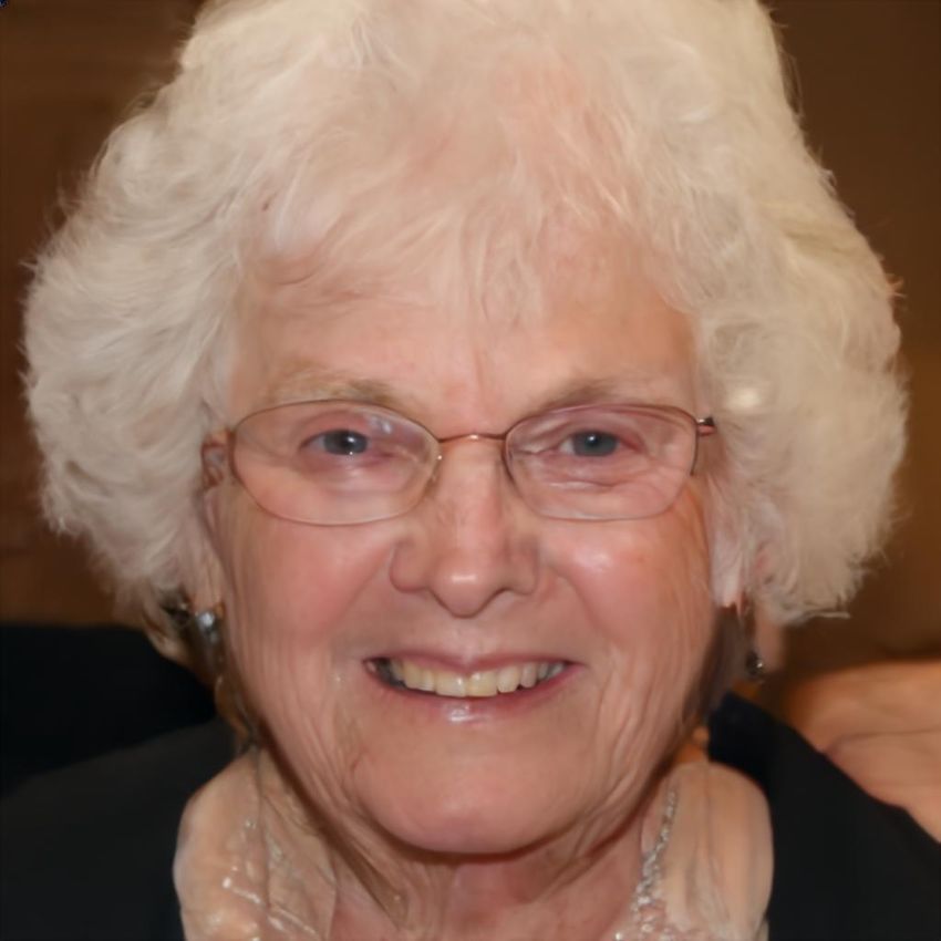
Bicubic              FSRGAN [7]          PULSE [28]        Regression          SR3

Figure 5: Comparison of different methods on the 16×16 → 128×128 face super-resolution task. Reference image has not been included
because of privacy concerns. Additional results in Appendix C.5.

    Fool rates (3 sec display w/ inputs, 16×16 → 128×128)                                 Fool rates (3 sec display w/ inputs, 64×64 → 256×256)
     FSRGAN            8.9%                                                              Regression              16.8%

       PULSE                          24.6%                                              SR3 (ours}                              38.8%
                                                                                                0      10    20     30     40     50     60     70
   Regression                                 29.3%

   SR3 (ours)                                                      54.1%                  Fool rates (3 sec display w/o inputs, 64×64 → 256×256)
            0     10          20       30         40     50        60      70
                                                                                         Regression            13.4%

   Fool rates (3 sec display w/o inputs, 16×16 → 128×128)                                SR3 (ours)                              39.0%
                                                                                                0      10    20     30     40     50     60     70
     FSRGAN            8.5%

       PULSE                                    33.7%                              Figure 7: ImageNet super-resolution fool rates (higher is better,
   Regression                 15.3%
                                                                                   photo-realistic samples yield a fool rate of 50%). SR3 and Regres-
                                                                                   sion outputs are compared against ground truth. (top) Subjects are
   SR3 (ours)                                              47.4%
            0     10          20       30         40     50        60      70
                                                                                   shown low-resolution inputs. (bottom) Inputs are not shown.

Figure 6: Face super-resolution human fool rates (higher is bet-
ter, photo-realistic samples yield a fool rate of 50%). Outputs of                 when asked solely about image quality in Task-2 (Fig. 6
4 models are compared against ground truth. (top) Subjects are                     (bottom)), the PULSE fool rate increases significantly.
shown low-resolution inputs. (bottom) Inputs are not shown.                            The fool rate for the Regression baseline is lower in
                                                                                   Task-2 (Fig. 6 (bottom)) than Task-1. The regression model
                                                                                   tends to generate images that are blurry, but nevertheless
image was not shown, so subjects only had to select the im-
                                                                                   faithful to the low resolution input. We speculate that in
age that was more photo-realistic. They were asked “Which
                                                                                   Task-1, given the inputs, subjects are influenced by consis-
image would you guess is from a camera?” Subjects viewed
                                                                                   tency, while in Task-2, ignoring consistency, they instead
images for 3 seconds before responding, in both tasks. The
                                                                                   focus on image sharpness. SR3 and Regression samples
source code for human evaluation can be found here 2 .
                                                                                   used for human evaluation are provided here 3 .
   The subject fool rate is the fraction of trials on which
                                                                                       We conduct similar human evaluation studies on natural
a subject selects the model output over ground truth. Our
                                                                                   images comparing SR3 and the regression baseline on Ima-
fool rates for each model are based on 50 subjects, each of
                                                                                   geNet. Figure 7 shows the results for Task-1 (top) and task-
whom were shown 50 of the 100 images in the test set. Fig-
                                                                                   2 (bottom). In both tasks with natural images, SR3 achieves
ure 6 shows the fool rates for Task-1 (top), and for Task-2
                                                                                   a human subject fool rate is close to 40%. Like the face
(bottom). In both experiments, the fool rate of SR3 is close
                                                                                   image experiments in Fig. 6, here again we find that the Re-
to 50%, indicating that SR3 produces images that are both
                                                                                   gression baseline yields a lower fool rate in Task-2, where
photo-realistic and faithful to the low-resolution inputs. We
                                                                                   the low resolution image is not shown. Again we speculate
find similar fool rates over a wide range of viewing dura-
                                                                                   that this is a result of a somewhat simpler task (looking at
tions up to 12 seconds.
                                                                                   2 rather than 3 images), and the fact that subjects can focus
   The fool rates for FSRGAN and PULSE in Task-1 are                               solely on image artifacts, such as blurriness, without having
lower than the Regression baseline and SR3. We speculate                           to worry about consistency between model output and the
that the PULSE optimization has failed to converge to high                         low resolution input.
resolution images sufficiently close to the inputs. Indeed,                            To further appreciate the experimental results it is use-
   2 https://tinyurl.com/sr3-human-eval-code                                             3 https://tinyurl.com/sr3-outputs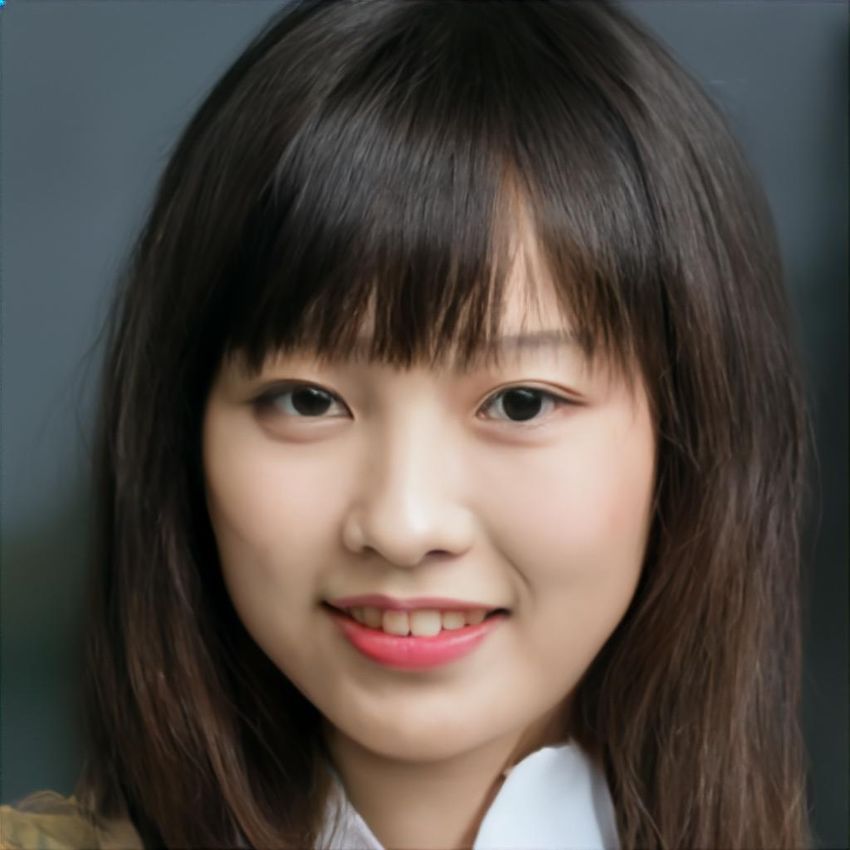
Model                              FID-50k
         Prior Work
           VQ-VAE-2 [39]                      38.1
           BigGAN (Truncation 1.0) [4]         7.4
           BigGAN (Truncation 1.5) [4]        11.8
         Our Work
           SR3 (Two Stage)                    11.3

 Table 4: FID scores for class-conditional 256×256 ImageNet.

ful to visually compare outputs of different models on the
same inputs, as in Figure 5. FSRGAN exhibits distortion in
face region and struggles with generating glasses properly
(e.g., top row). It also fails to recover texture details in the
hair region (see bottom row). PULSE often produces im-
ages that differ significantly from the input image, both in
the shape of the face and the background, and sometimes
in gender too (see bottom row) presumably due to failure
of the optimization to find a sufficiently good minima. As
noted above, our Regression baseline produces results con-
sistent to the input, however they are typically quite blurry.
By comparison, the SR3 results are consistent with the input
and contain more detailed image structure.
4.3. Cascaded High-Resolution Image Synthesis
    We study cascaded image generation, where SR3 models
at different scales are chained together with unconditional
generative models, enabling high-resolution image synthe-
sis. Cascaded generation allows one to train different mod-
els in parallel, and each model in the cascade solves a sim-
pler task, requiring fewer parameters and less computation         Figure 8: Synthetic 1024×1024 face images. We first sample
for training. Inference with cascaded models is also more          from an unconditional 64×64 diffusion model, then pass the sam-
efficient, especially for iterative refinement models. With        ples through two 4× SR3 models, i.e., 64×64 → 256×256 →
cascaded generation we found it effective to use more re-          1024×1024. Additional samples in Appendix C.7, C.8 and C.9.
finement steps at low-resolutions, and fewer steps at higher
resolutions. This was much more efficient than generating
directly at high resolution without sacrificing image quality.     currently trained cascaded generation models using super-
    We train a DDPM [17] model for unconditional 64×64             resolution conditioned on class labels (our super-resolution
face generation. Samples from this model are then fed to           is not conditioned on class labels), and observed a similar
two 4× SR3 models, up-sampling to 2562 and then to 10242           trend in FID scores. The effectiveness of cascaded image
pixels. Synthetic high-resolution face samples are shown in        generation indicates that SR3 models are robust to the pre-
Figure 8. In addition, we train an Improved DDPM [30]              cise distribution of inputs (i.e., the specific form of anti-
model on class-conditional 64×64 ImageNet, and we pass             aliasing and downsampling).
its generated samples to a 4× SR3 model yielding 2562 pix-             Ablation Studies: Table 5 shows ablation studies on our
els. The 4× SR3 model is not conditioned on the class label.       64 × 64 → 256 × 256 Imagenet SR3 model. In order to im-
See Figure 9 for representative samples.                           prove the robustness of the SR3 model, we experiment with
    Table 4 reports FID scores for the resulting class-            use of data augmentation while training. Specifically, we
conditional ImageNet samples. Our 2-stage model im-                trained the model with varying amounts of Gaussian Blur-
proves on VQ-VAE-2 [39], is comparable to deep BigGANs             ring noise added to the low resolution input image. No
[4] at truncation factor of 1.5 but underperforms them a           blurring is applied during inference. We find that this has
truncation factor of 1.0. Unlike BigGAN, our diffusion             a siginificant impact, improving the FID score roughly by 2
models do not provide a knob to control sample quality vs.         points. We also explore the choice of Lp norm for the de-
sample diversity, and finding ways to do so is interesting         noising objective (Equation 6). We find that L1 norm gives
avenue for future research. Nichol and Dhariwal [30] con-          slightly better FID scores than L2 .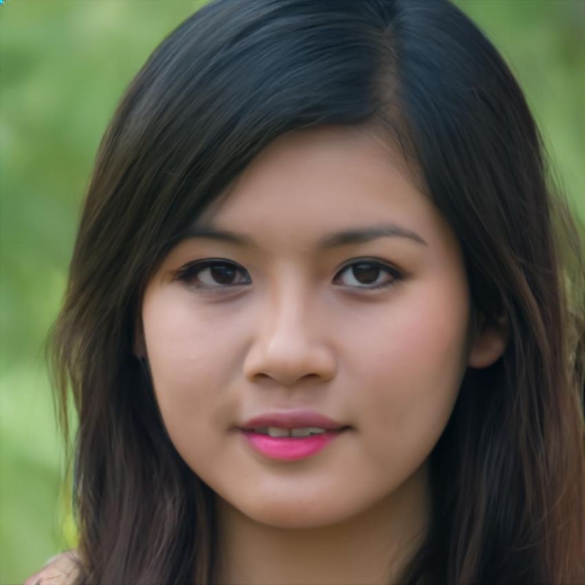
images, as well as unconditional samples when cascaded
                                                                  with a unconditional model. We demonstrate SR3 on
                                                                  face and natural image super-resolution at high resolution
                                                                  and high magnification ratios (e.g., 64×64→256×256 and
                                                                  256×256→1024×1024). SR3 achieves a human fool rate
                                                                  close to 50%, suggesting photo-realistic outputs.

                                                                  Acknowledgements
                                                                     We thank Jimmy Ba, Adji Bousso Dieng, Chelsea Finn,
                                                                  Geoffrey Hinton, Natacha Mainville, Shingai Manjengwa,
                                                                  and Ali Punjani for providing their face images on which
                                                                  we demonstrate the face SR3 results. We thank Ben Poole,
                                                                  Samy Bengio and the Google Brain team for research dis-
                                                                  cussions and technical assistance. We also thank authors
                                                                  of [28] for generously providing us with baseline super-
                                                                  resolution samples for human evaluation.

                                                                  References
                                                                   [1] Namhyuk Ahn, Byungkon Kang, and Kyung-Ah Sohn. Im-
                                                                       age Super-resolution via Progressive Cascading Residual
Figure 9: Synthetic 256×256 ImageNet images. We first draw             Network. In CVPR, 2018.
a random label, then sample a 64×64 image from a class-            [2] Martin Arjovsky, Soumith Chintala, and Léon Bottou.
conditional diffusion model, and apply a 4× SR3 model to obtain        Wasserstein GAN. In arXiv, 2017.
256×256 images. Additional samples in Appendix C.10 and C.11.      [3] David Berthelot, Peyman Milanfar, and Ian Goodfellow.
                                                                       Creating high resolution images with a latent adversarial
                                                                       generator. arXiv preprint 2003.02365, 2020.
          Model                           FID-50k
                                                                   [4] Andrew Brock, Jeff Donahue, and Karen Simonyan. Large
          Training with Augmentation                                   scale GAN training for high fidelity natural image synthesis.
            SR3                             13.1                       arXiv preprint arXiv:1809.11096, 2018.
            SR3 (w/ Gaussian Blur)          11.3                   [5] Ruojin Cai, Guandao Yang, Hadar Averbuch-Elor, Zekun
          Objective Lp Norm                                            Hao, Serge Belongie, Noah Snavely, and Bharath Hariharan.
           SR3 (L2 )                        11.8                       Learning Gradient Fields for Shape Generation. In ECCV,
           SR3 (L1 )                        11.3                       2020.
                                                                   [6] Nanxin Chen, Yu Zhang, Heiga Zen, Ron J. Weiss, Moham-
Table 5: Ablation study on SR3 model for class-conditional             mad Norouzi, and William Chan. WaveGrad: Estimating
256×256 ImageNet.                                                      Gradients for Waveform Generation. In ICLR, 2021.
                                                                   [7] Yu Chen, Ying Tai, Xiaoming Liu, Chunhua Shen, and Jian
5. Discussion and Conclusion                                           Yang. Fsrnet: End-to-end learning face super-resolution with
                                                                       facial priors. In Proc. IEEE Conference on Computer Vision
    Bias is an important problem in all generative models.             and Pattern Recognition, pages 2492–2501, 2018.
SR3 is no different, and suffers from bias issues. While in        [8] Ryan Dahl, Mohammad Norouzi, and Jonathon Shlens. Pixel
theory, our log-likelihood based objective is mode cover-              recursive super resolution. In ICCV, 2017.
ing (e.g., unlike some GAN-based objectives), we believe           [9] Emily Denton, Soumith Chintala, Arthur Szlam, and Rob
it is likely our diffusion-based models drop modes. We ob-             Fergus. Deep Generative Image Models using a Laplacian
served some evidence of mode dropping, the model consis-               Pyramid of Adversarial Networks. In NIPS, 2015.
tently generates nearly the same image output during sam-         [10] Laurent Dinh, Jascha Sohl-Dickstein, and Samy Bengio.
pling (when conditioned on the same input). We also ob-                Density estimation using real NVP. arXiv:1605.08803,
served the model to generate very continuous skin texture in           2016.
                                                                  [11] Chao Dong, Chen Change Loy, Kaiming He, and Xiaoou
face super-resolution, dropping moles, pimples and pierc-
                                                                       Tang. Learning a deep convolutional network for image
ings found in the reference. SR3 should not be used for
                                                                       super-resolution. In European conference on computer vi-
any real world super-resolution tasks, until these biases are          sion, pages 184–199. Springer, 2014.
thoroughly understood and mitigated.                              [12] Chao Dong, Chen Change Loy, Kaiming He, and Xiaoou
    In conclusion, SR3 is an approach to image super-                  Tang. Image super-resolution using deep convolutional net-
resolution via iterative refinement. SR3 can be used in a cas-         works. IEEE transactions on pattern analysis and machine
caded fashion to generate high resolution super-resolution             intelligence, 38(2):295–307, 2015.
[13] Chao Dong, Chen Change Loy, and Xiaoou Tang. Acceler- [30] Alex Nichol and Prafulla Dhariwal. Improved de-
ating the super-resolution convolutional neural network. In noising diffusion probabilistic models. arXiv preprint
European conference on computer vision, pages 391–407. arXiv:2102.09672, 2021.
Springer, 2016. [31] Aäron van den Oord, Sander Dieleman, Heiga Zen, Karen
[14] Ian J Goodfellow, Jean Pouget-Abadie, Mehdi Mirza, Bing Simonyan, Oriol Vinyals, Alex Graves, Nal Kalchbren-
Xu, David Warde-Farley, Sherjil Ozair, Aaron Courville, and ner, Andrew Senior, and Koray Kavukcuoglu. WaveNet:
Yoshua Bengio. Generative Adversarial Networks. NIPS, A Generative Model for Raw Audio. arXiv preprint
2014. arXiv:1609.03499, 2016.
[15] Ishaan Gulrajani, Faruk Ahmed, Martin Arjovsky, Vincent [32] Aäron van den Oord, Nal Kalchbrenner, Oriol Vinyals, Lasse
Dumoulin, and Aaron Courville. Improved training of Espeholt, Alex Graves, and Koray Kavukcuoglu. Condi-
wasserstein gans. arXiv preprint arXiv:1704.00028, 2017. tional Image Generation with PixelCNN Decoders. In NIPS,
[16] Kaiming He, Xiangyu Zhang, Shaoqing Ren, and Jian Sun. 2016.
Deep residual learning for image recognition. In Proceed- [33] Niki Parmar, Ashish Vaswani, Jakob Uszkoreit, Lukasz
ings of the IEEE conference on computer vision and pattern Kaiser, Noam Shazeer, Alexander Ku, and Dustin Tran. Im-
recognition, pages 770–778, 2016. age transformer. In International Conference on Machine
[17] Jonathan Ho, Ajay Jain, and Pieter Abbeel. Denoising diffu- Learning, 2018.
sion probabilistic models. In NeurIPS, 2020. [34] Ethan Perez, Florian Strub, Harm De Vries, Vincent Du-
[18] Aapo Hyvärinen and Peter Dayan. Estimation of non- moulin, and Aaron Courville. FiLM: Visual Reasoning with
normalized statistical models by score matching. JMLR, a General Conditioning Layer . In AAAI, 2018.
6(4), 2005. [35] Eduardo Pérez-Pellitero, Jordi Salvador, J. Hidalgo, and B.
[19] Tero Karras, Timo Aila, Samuli Laine, and Jaakko Lehtinen. Rosenhahn. Psyco: Manifold span reduction for super reso-
Progressive growing of gans for improved quality, stability, lution. 2016 IEEE Conference on Computer Vision and Pat-
and variation. In ICLR, 2018. tern Recognition (CVPR), pages 1837–1845, 2016.
[36] Alec Radford, Luke Metz, and Soumith Chintala. Un-
[20] Tero Karras, Samuli Laine, and Timo Aila. A Style-
supervised representation learning with deep convolu-
Based Generator Architecture for Generative Adversarial
tional generative adversarial networks. arXiv preprint
Networks. In CVPR, 2019.
arXiv:1511.06434, 2015.
[21] Jiwon Kim, Jung Kwon Lee, and Kyoung Mu Lee. Accurate
[37] Martin Raphan and Eero P Simoncelli. Least squares esti-
image super-resolution using very deep convolutional net-
mation without priors or supervision. Neural computation,
works. In CVPR, 2016.
23(2):374–420, 2011.
[22] Jiwon Kim, Jung Kwon Lee, and Kyoung Mu Lee. Deeply-
[38] Suman Ravuri and Oriol Vinyals. Classification accuracy
recursive convolutional network for image super-resolution.
score for conditional generative models. arXiv preprint
In Proceedings of the IEEE conference on computer vision
arXiv:1905.10887, 2019.
and pattern recognition, pages 1637–1645, 2016.
[39] Ali Razavi, Aaron van den Oord, and Oriol Vinyals. Gen-
[23] Diederik P. Kingma and Prafulla Dhariwal. Glow: Genera- erating diverse high-fidelity images with vq-vae-2. arXiv
tive Flow with Invertible 1x1 Convolutions. In NIPS, 2018. preprint arXiv:1906.00446, 2019.
[24] Diederik P Kingma and Max Welling. Auto-Encoding Vari- [40] Danilo Rezende and Shakir Mohamed. Variational inference
ational Bayes. In ICLR, 2013. with normalizing flows. In International Conference on Ma-
[25] Christian Ledig, Lucas Theis, Ferenc Huszár, Jose Caballero, chine Learning, pages 1530–1538. PMLR, 2015.
Andrew Cunningham, Alejandro Acosta, Andrew Aitken, [41] Danilo Jimenez Rezende, Shakir Mohamed, and Daan Wier-
Alykhan Tejani, Johannes Totz, Zehan Wang, et al. Photo- stra. Stochastic backpropagation and approximate inference
realistic single image super-resolution using a generative ad- in deep generative models. In International conference on
versarial network. In ICCV, 2017. machine learning, pages 1278–1286. PMLR, 2014.
[26] Rafał K Mantiuk, Anna Tomaszewska, and Radosław Man- [42] Olaf Ronneberger, Philipp Fischer, and Thomas Brox. U-
tiuk. Comparison of four subjective methods for image qual- net: Convolutional networks for biomedical image segmen-
ity assessment. In Computer graphics forum, volume 31, tation. In International Conference on Medical image com-
pages 2478–2491. Wiley Online Library, 2012. puting and computer-assisted intervention, 2015.
[27] Jacob Menick and Nal Kalchbrenner. Generating High Fi- [43] Olga Russakovsky, Jia Deng, Hao Su, Jonathan Krause, San-
delity Images with Subscale Pixel Networks and Multidi- jeev Satheesh, Sean Ma, Zhiheng Huang, Andrej Karpathy,
mensional Upscaling. In ICLR, 2019. Aditya Khosla, Michael Bernstein, et al. Imagenet large
[28] Sachit Menon, Alexandru Damian, Shijia Hu, Nikhil Ravi, scale visual recognition challenge. International journal of
and Cynthia Rudin. PULSE: Self-supervised photo upsam- computer vision, 115(3):211–252, 2015.
pling via latent space exploration of generative models. In [44] Mehdi SM Sajjadi, Bernhard Scholkopf, and Michael
CVPR, 2020. Hirsch. Enhancenet: Single image super-resolution through
[29] Luke Metz, Ben Poole, David Pfau, and Jascha Sohl- automated texture synthesis. In Proceedings of the IEEE
Dickstein. Unrolled generative adversarial networks. arXiv International Conference on Computer Vision, pages 4491–
preprint arXiv:1611.02163, 2016. 4500, 2017.[45] Tim Salimans, Andrej Karpathy, Xi Chen, and Diederik P [61] Lingbo Yang, Chang Liu, Pan Wang, Shanshe Wang, Peiran
Kingma. PixelCNN++: Improving the PixelCNN with dis- Ren, Siwei Ma, and Wen Gao. HiFaceGAN: Face Renova-
cretized logistic mixture likelihood and other modifications. tion via Collaborative Suppression and Replenishment. In
In International Conference on Learning Representations, arXiv, 2020.
2017. [62] Jason J. Yu, Konstantinos G. Derpanis, and Marcus A.
[46] Saeed Saremi, Arash Mehrjou, Bernhard Schölkopf, and Brubaker. Wavelet Flow: Fast Training of High Resolution
Aapo Hyvärinen. Deep Energy Estimator Networks. arXiv Normalizing Flows. In arXiv, 2020.
preprint arXiv:1805.08306, 2018. [63] Richard Zhang, Phillip Isola, and Alexei A Efros. Colorful
[47] Jascha Sohl-Dickstein, Eric Weiss, Niru Maheswaranathan, image colorization. In ECCV, 2016.
and Surya Ganguli. Deep unsupervised learning using [64] Yulun Zhang, Kunpeng Li, Kai Li, Lichen Wang, Bineng
nonequilibrium thermodynamics. In ICML, pages 2256– Zhong, and Yun Fu. Image super-resolution using very
2265. PMLR, 2015. deep residual channel attention networks. In Proceedings of
[48] Jascha Sohl-Dickstein, Eric A. Weiss, Niru Mah- the European conference on computer vision (ECCV), pages
eswaranathan, and Surya Ganguli. Deep Unsupervised 286–301, 2018.
Learning using Nonequilibrium Thermodynamics. In ICML,
2015.
[49] Yang Song and Stefano Ermon. Generative Modeling by
Estimating Gradients of the Data Distribution. In NeurIPS,
2019.
[50] Yang Song and Stefano Ermon. Improved Techniques for
Training Score-Based Generative Models. arXiv preprint
arXiv:2006.09011, 2020.
[51] Yang Song, Jascha Sohl-Dickstein, Diederik P. Kingma, Ab-
hishek Kumar, Stefano Ermon, and Ben Poole. Score-Based
Generative Modeling through Stochastic Differential Equa-
tions. In ICLR, 2021.
[52] Ilya Sutskever, Oriol Vinyals, and Quoc Le. Sequence to
Sequence Learning with Neural Networks. In NIPS, 2014.
[53] Ying Tai, Jian Yang, and Xiaoming Liu. Image super-
resolution via deep recursive residual network. In Proceed-
ings of the IEEE conference on computer vision and pattern
recognition, pages 3147–3155, 2017.
[54] Arash Vahdat and Jan Kautz. NVAE: A deep hierarchical
variational autoencoder. In NeurIPS, 2020.
[55] Aaron van den Oord, Nal Kalchbrenner, and Koray
Kavukcuoglu. Pixel recurrent neural networks. International
Conference on Machine Learning, 2016.
[56] Aaron van den Oord, Nal Kalchbrenner, Oriol Vinyals, Lasse
Espeholt, Alex Graves, and Koray Kavukcuoglu. Condi-
tional image generation with PixelCNN decoders. In Ad-
vances in Neural Information Processing Systems, pages
4790–4798, 2016.
[57] Ashish Vaswani, Noam Shazeer, Niki Parmar, Jakob Uszko-
reit, Llion Jones, Aidan N. Gomez, Lukasz Kaiser, and Illia
Polosukhin. Attention Is All You Need. In NIPS, 2017.
[58] Pascal Vincent. A connection between score matching and
denoising autoencoders. Neural Computation, 23(7):1661–
1674, 2011.
[59] Zhou Wang, A.C. Bovik, H.R. Sheikh., and E.P. Simon-
celli. Image quality assessment: from error visibility to struc-
tural similarity. IEEE Transactions on Image Processing,
13(4):600–612, 2004.
[60] Zhaowen Wang, Ding Liu, Jianchao Yang, Wei Han, and
Thomas Huang. Deep networks for image super-resolution
with sparse prior. In Proceedings of the IEEE international
conference on computer vision, pages 370–378, 2015.Appendix
This appendix includes further details about the architecture of the models used for super-resolution. It also formulates
the training objective in terms of a variation bound and in terms of denoising score-matching. We then provide additional
experimental results to complement those in the main body of the paper.
A. Task Specific Architectural Details
Table A.1 summarizes the primary architecture details for each super-resolution task. For a particular task, we use the same
architecture for both SR3 and Regression models. Figure A.1 describes our method of conditioning the diffusion model
on the low resolution image. We first interpolate the low resolution image to the target high resolution, and then simply
concatenate it with the input noisy high resolution image.
Task Channel Dim Depth Multipliers # ResNet Blocks # Parameters
16 × 16 → 128 × 128 128 {1, 2, 4, 8, 8} 3 550M
64 × 64 → 256 × 256 128 {1, 2, 4, 4, 8, 8} 3 625M
64 × 64 → 512 × 512 64 {1, 2, 4, 8, 8, 16, 16} 3 625M
256 × 256 → 1024 × 1024 16 {1, 2, 4, 8, 16, 32, 32, 32} 2 150M
Table A.1: Task specific architecture hyper-parameters for the U-Net model. Channel Dim is the dimension of the first U-Net layer, while
the depth multipliers are the multipliers for subsequent resolutions.
82 , 1024 82 , 1024
642 , 256 642 , 256
x · yt 1282 , 128 1282 , 128 yt−1
Figure A.1: Description of the U-Net architecture with skip connections. The low resolution input image x is interpolated to the target
high resolution, and concatenated with the noisy high resolution image yt . We show the activation dimensions for the example task of
16×16 → 128×128 super resolution.
B. Justification of the Training Objective
B.1. A Variational Bound Perspective
Following Ho et al. [17], we justify the choice of the training objective in (6) for the probabilistic model outlined in (9)
from a variational lower bound perspective. If the forward diffusion process is viewed as a fixed approximate posterior to the
inference process, one can derive the following variational lower bound on the marginal log-likelihood:
X pθ (yt−1 |yt , x)
E(x,y0 ) log pθ (y0 |x) ≥ Ex,y0 Eq(y1:T |y0 ) log p(yT ) + log . (12)
q(yt |yt−1 )
t≥1Given the particular parameterization of the inference process outlined above, one can show [17] that the negative varia-
tional lower bound can be expressed as the following simplified loss, up to a constant weighting of each term for each time
step:
T 2
X 1 √ p
Ex,y0 , − θ (x, γt y0 + 1 − γt , γt ) (13)
t=1
T 2
where ∼ N (0, I). Note that this objective function corresponds to L2 norm in (6), and a characterization of p(γ) in terms
of a uniform distribution over {γ1 , . . . , γT }.
B.2. A Denoising Score-Matching Perspective
Our approach is also linked to denoising score matching [18, 58, 37, 46] for training unnormalized energy functions for
density estimation. These methods learn a parametric score function to approximate the gradient of the empirical data log-
density. To make sure that the gradient of the data log-density is well-defined, one often replaces each data point with a
Gaussian distribution with a small variance. Song and Ermon [50] advocate for the use of a Multi-scale Guassian mixture as
the target density, where each data point is perturbed with different amounts of Gaussian noise, so that Langevin dynamics
starting from pure noise can still yield reasonable samples.
One can view our approach as a variant of denoising score matching in which the target density is given by a mixture of
√
y |y0 , γ) = N (e
q(e y | γy0 , 1 − γ) for different values of y0 and γ. Accordingly, the gradient of data log-density is given by
√
y | y0 , γ)
d log q(e ye − γy0
= − √ = −, (14)
dey 1−γ
which is used as the regression target of our model.
C. Additional Experimental Results
The following figures show more examples of SR3 on faces, natural images, and samples from unconditional generative
models, architectural details, more details about the formulation of the loss. We first show more examples of SR3, augmenting
the results shown in Figures 4, 3, 5. We then show cascaded generation of 1024 × 1024 face images, followed by more
unconditional samples for 1024 × 1024 faces, and 256 × 256 class conditional ImageNet samples.Face Super-Resolution 64×64 → 512×512
Bicubic Regression SR3 (ours) Reference
Figure C.1: Additional results of a SR3 model (64×64 → 512×512), trained on FFHQ, and applied to images outside of the training set.
We crop and align these faces to be consistent with FFHQ using the script provided here.Bicubic Regression SR3 (ours) Reference Figure C.2: Additional results of a SR3 model (64×64 → 512×512), trained on FFHQ, and applied to images outside of the training set. We crop and align these faces to be consistent with FFHQ using the script provided here.
Natural Image Super-Resolution 64×64 → 256×256
                   Bicubic                 Regression                SR3 (ours)                Reference

Figure C.3: Additional results of a SR3 model (64×64 → 256×256), trained on ImageNet and evaluated on ImageNet test images.
Bicubic Regression SR3 (ours) Reference Figure C.4: Additional results of a SR3 model (64×64 → 256×256), trained on ImageNet and evaluated on ImageNet test images.
Benchmark Comparison on Test Faces 16×16 → 128×128
                      Bicubic          FSRGAN [7]          PULSE [28]          Regression             SR3

Figure C.5: Additional results showing the comparison between different methods on the 16×16 → 128×128 face super-resolution task.
Cascaded Face Generation 1024×1024
(64×64) (256×256) (1024×1024)
Figure C.6: Cascaded generation on faces using an unconditional model chained with two SR3 models.Unconditional Face Samples 1024×1024 Figure C.7: Additional Synthetic 1024×1024 faces images. We first sample from an unconditional 64×64 diffusion model, then pass the samples through two 4× SR3 models, i.e., 64×64 → 256×256 → 1024×1024.
Figure C.8: Additional Synthetic 1024×1024 faces images. We first sample from an unconditional 64×64 diffusion model, then pass the
samples through two 4× SR3 models, i.e., 64×64 → 256×256 → 1024×1024.
You can also read