Leaf area index in Earth system models: how the key variable of vegetation seasonality works in climate projections
←
→
Page content transcription
If your browser does not render page correctly, please read the page content below
LETTER • OPEN ACCESS

Leaf area index in Earth system models: how the key variable of
vegetation seasonality works in climate projections
To cite this article: Hoonyoung Park and Sujong Jeong 2021 Environ. Res. Lett. 16 034027

View the article online for updates and enhancements.

                              This content was downloaded from IP address 46.4.80.155 on 19/09/2021 at 10:53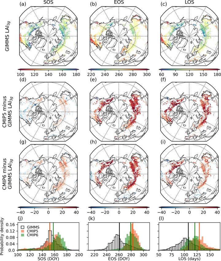
Environ. Res. Lett. 16 (2021) 034027 https://doi.org/10.1088/1748-9326/abe2cf
LETTER
Leaf area index in Earth system models: how the key variable of
OPEN ACCESS
vegetation seasonality works in climate projections
RECEIVED
28 August 2020 Hoonyoung Park1,2 and Sujong Jeong1,2
REVISED 1
17 January 2021 Department of Environmental Planning, Graduate School of Environmental Studies, Seoul National University, Seoul, Republic of
Korea
ACCEPTED FOR PUBLICATION 2
3 February 2021
Institute for Sustainable Development (ISD), Seoul National University, Seoul, Republic of Korea
PUBLISHED E-mail: sujong@snu.ac.kr
22 February 2021
Keywords: CMIP5, CMIP6, Earth system models, leaf area index, vegetation seasonality, vegetation phenology
Original content from Supplementary material for this article is available online
this work may be used
under the terms of the
Creative Commons
Attribution 4.0 licence. Abstract
Any further distribution Earth system models (ESMs) are widely used in scientific research to understand the responses of
of this work must
maintain attribution to various components of Earth systems to natural and anthropogenic forcings. ESMs embody
the author(s) and the title terrestrial ecosystems on the basis of the leaf area index (LAI) to formulate various interactions
of the work, journal
citation and DOI. between the land surface and atmosphere. Here, we evaluated the LAI seasonality of deciduous
forests simulated by 14 ESMs participating in the Coupled Model Intercomparison Project Phase 5
(CMIP5) and CMIP6 to understand the efficacy of recent ESMs in describing leaf dynamics in the
northern extratropics from 1982 to 2014. We examined three indicators of LAI seasonality (annual
mean, amplitude, and phase) and three phenological dates (start (SOS), end (EOS), and length of
growing season (LOS)) of the models in comparison to the third-generation LAI of Global
Inventory Modeling and Mapping Studies (GIMMS LAI3g ) and the Climate Research Unit gridded
time series dataset. CMIP6 models tend to simulate larger annual means (1.7 m2 m−2 ), weaker
amplitudes (0.9 m2 m−2 ), and delayed phases (226 DOY) compared to the GIMMS LAI3g
(1.2 m2 m−2 , 1.2 m2 m−2 , and 212 DOY, respectively), yet are similar to the CMIP5 models
(2.2 m2 m−2 , 1.0 m2 m−2 , and 225 DOY). The later phase is attributed to a systematic positive bias
in EOS of the CMIP5 and CMIP6 models (later by 22 and 18 d, respectively) compared to the
GIMMS LAI3g (261 DOY). Further tests on phenological responses to seasonal temperature
revealed that the majority of CMIP5 and CMIP6 ESMs inaccurately describe the sensitivities of
SOS and EOS to seasonal temperature and the recent changes in mean SOS and EOS distributions
(2005–2014 minus 1982–1991). This study suggests that phenology schemes of deciduous forests,
especially for autumn leaf senescence, should be revisited to achieve an accurate representation of
terrestrial ecosystems and their interactions.
1. Introduction adjusts the surface energy balance, the hydrological
cycle, the carbon budget, and boundary-layer meteor-
Mid- and high-latitude vegetation shows clear sea- ology (Bonan 2008, Jeong et al 2009, Lee et al 2011,
sonality in canopy structure from spring emergence Richardson et al 2013, Piao et al 2020a, 2020b, Jeong
to autumn senescence, in accordance with seasonal and Park 2020) (figure 1). ESMs utilize LAI to rep-
changes in environmental conditions (Richardson resent these complicated and dynamic processes that
et al 2013, Piao et al 2020a). In Earth system mod- occur in terrestrial ecosystems, analyzing responses
els (ESMs), canopy structure is parameterized by leaf to environmental conditions, and adjusting surface
area index (LAI), which describes changes in the can- interactions with the Earth system. The dynamic rep-
opy structure resulting from surface interactions with resentation of the LAI in ESMs enables the prognostic
the environment (Arora and Boer 2005). In addi- simulation of terrestrial carbon fluxes and their influ-
tion, LAI is also the key variable controlling the mag- ence on the concentration of atmospheric CO2 , which
nitude of biosphere–climate interactions because it is necessary for carrying out concentration-driven
© 2021 The Author(s). Published by IOP Publishing Ltd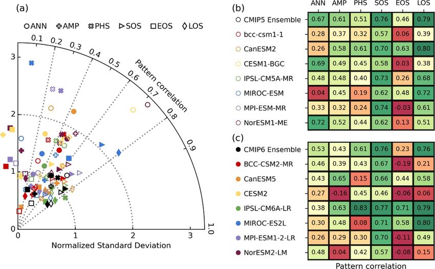
Environ. Res. Lett. 16 (2021) 034027                                                                           H Park and S Jeong

                          Figure 1. Schematic diagram of the role of LAI and its major interactions in ESMs.

ESM experiments with a fully coupled carbon cycle                   ESMs of Coupled Model Intercomparison Project
(Hurrell et al 2013, Eyring et al 2016). Thus, an accur-            Phase 5 (CMIP5) (later onset and offset by 6 and
ate representation of LAI seasonality in the models is              36 d, respectively; Anav et al 2013). This inaccurate
necessary for realistic simulations of terrestrial eco-             representation of LAI dynamics disrupts energy bal-
system dynamics and the corresponding interactions                  ances, hydrological cycles, and carbon fluxes on the
with the surrounding environment in climate simu-                   land surface in the model (Richardson et al 2013,
lations.                                                            Zhao et al 2020). Considering the role of vegeta-
    Vegetation seasonality remains a challenging                    tion phenology and its ramifications (Peñuelas et al
topic in ESM research, primarily because of the highly              2009), accurate simulations of vegetation seasonal-
intricate nature of vegetation phenology (Arora                     ity are a prerequisite for creating a more accurate
and Boer 2005, Richardson et al 2012). Despite the                  representation of past, present, and future climate
inherent complexities of various phenological pro-                  systems.
cesses, there have been numerous advances in veget-                      Modeling groups and various institutes world-
ation seasonality modeling, from prescribed seasonal                wide have endeavored to improve ESMs on the basis
changes to dynamic phenology that is highly respons-                of the CMIP. CMIPs were initiated to broaden our
ive to the simulation of meteorological conditions                  understanding of the climate system and its changes
(Schwartz 2003). Currently, most ESMs describe the                  by natural and anthropogenic forcing in a multi-
seasonal cycle of vegetation activity using process-                model context. During the last two decades, three
based approaches. However, in current ESMs, the                     generations of CMIPs (CMIP3, CMIP4, and CMIP5)
simulation of LAI seasonality is not yet sufficiently               have produced standardized and publicly available
accurate to describe the Earth system. Several studies              multi-model outputs, opening a new horizon in cli-
have found that simulations of vegetation seasonality               mate science by yielding numerous contributions to
frequently display delayed or prolonged growing sea-                model evaluations, improvements in the field of phys-
sons, especially for site-based models (earlier onset               ics, and future climate projections (Stocker et al 2013,
of 10 d over North America; Richardson et al 2012),                 Eyring et al 2016). As a continuation of CMIP5, the
uncoupled land surface models (later onset and offset               development of CMIP6 is ongoing in order to pro-
of 20 and 44 d, respectively, over the Northern Hemi-               mote our understanding of Earth systems (Eyring et al
sphere; Murray-Tortarolo et al 2013), and coupled                   2016). The latest ESMs participating in CMIP6 have

                                                      2
Environ. Res. Lett. 16 (2021) 034027                                                                 H Park and S Jeong

applied improved physics regarding the atmosphere,                We used a 1 km global land cover classifica-
ocean, and land surface (Hajima et al 2020, Mauritsen        tion dataset, generated by the Department of Geo-
et al 2019, Arora et al 2020, Boucher et al 2020,            graphy at the University of Maryland (UMd) (Hansen
Danabasoglu et al 2020, Mudryk et al 2020, Seland            et al 2000), to confine our data analysis to natural
et al 2020), which in turn may enhance the perform-          deciduous forests in the northern mid- and high-
ance of LAI seasonality simulations. The evaluation of       latitude regions (>30◦ N). Natural deciduous forests
CMIP6 LAI outputs by comparing them with the pre-            are classified into the following categories: decidu-
vious CMIP5 LAI and remotely sensed LAI datasets             ous needleleaf forest, deciduous broadleaf forest,
(e.g. Global Inventory Modeling and Mapping Stud-            mixed forest, and woodland. We utilized the near-
ies (GIMMS) LAI3g ) can illustrate recent improve-           surface (2 m) air temperature of the CRU TS4.01 cli-
ments in the simulated LAI seasonality, highlighting         mate dataset to identify the response of phenological
the remaining deficiencies of LAI simulation in the          dates to air temperature for the GIMMS LAI3g data-
latest ESMs. Therefore, the evaluation of the CMIP6          set. CRU TS4.01 is a high-resolution (0.5◦ latitude–
LAI seasonality is crucial to finding the key to further     longitude grid) monthly climate dataset that covers all
improve LAI dynamics.                                        land areas, excluding Antarctica, from 1901 to 2016
     This study evaluated the LAI seasonality that           (Harris et al 2020). It provides a credible climate
was simulated in the CMIP6 ESMs in comparison                dataset based on networks of surface weather station
with the CMIP5 ESMs outputs and remotely sensed              observations and is thus appropriate for examining
GIMMS LAI3g for deciduous forests over the north-            changes in seasonal temperature.
ern extratropics (>30◦ N) from 1982 to 2014. First,               We used the monthly LAI and near-surface air
we compared the LAI seasonality in the CMIP5 and             temperature outputs of a total of 14 models, with
CMIP6 ESMs to the GIMMS LAI3g with regard to                 seven models participating in the CMIP5 and the
three seasonal indicators (annual mean, amplitude,           remaining seven latest model versions participat-
and phase) and three phenological dates (start, end,         ing in the CMIP6 (tables 1 and 2). By comparing
and length of the growing season; SOS, EOS, and LOS,         the characteristics of the seven pairs of CMIP5 and
respectively). In addition, we examined the interan-         CMIP6 models, we aimed to present the improve-
nual sensitivities and long-term responses of phen-          ments in vegetation seasonality in the CMIP6 mod-
ological dates to seasonal temperature variations in         els, as compared to the previous CMIP. We analyzed
the CMIP5 and CMIP6 ESMs compared with the                   near-surface air temperature and LAI from 1982 to
GIMMS LAI3g and Climate Research Unit (CRU)                  2014, which is the period of overlap among the CRU
TS4.01 near-surface air temperature. By illustrating         TS4.01 (1901–2016), GIMMS LAI3g (1982–2016),
biases in the mean patterns and temperature sensit-          and CMIP6 historical scenario outputs (1850–2014).
ivities, this study addresses the recent improvements        Historical simulations are driven by observation-
and current challenges of the simulation of LAI sea-         based forcing, such as greenhouse gas concentration,
sonality in CMIP6 ESMs.                                      gridded land-use data, volcanic aerosols, sea surface
                                                             temperature, and sea ice concentrations (Eyring et al
2. Data and methods                                          2016), thus allowing the comparison of ESM simula-
                                                             tions with observed changes in the climate system. In
2.1. Data                                                    the case of CMIP5, the historical scenario only spans
This study used the GIMMS LAI3g v4 dataset as the            from 1850 to 2005, which is 9 year shorter period
observational data to evaluate the simulated LAI in          than the CMIP6 historical scenario. To ensure the
ESMs. GIMMS LAI3g is the longest available satellite         maximum overlap in the CMIP6, CRU TS4.01, and
LAI dataset (1982–2016), which covers the entirety of        GIMMS LAI3g outputs, we supplemented the 9 year
the Earth’s surface with a high spatiotemporal resolu-       period (2006–2014) of missing data with the output
tion (1/12◦ and 15 d intervals) (Zhu et al 2013). Along      of representative concentration pathway 8.5 (RCP8.5)
with its long-term data, GIMMS LAI3g acquires its            scenario in line with previous studies (Quetin and
high quality by multi-sensor-based bias corrections          Swann 2018, Mudryk et al 2020). This is justified by
and 15 d maximum composites to alleviate the influ-          the finding that the RCP8.5 scenario closely (within
ence of non-vegetative effects. In addition, it substi-      1% for 2005–2020) tracks anthropogenic greenhouse
tutes possibly contaminated LAI data with snow or            gas emissions (Schwalm et al 2020).
cloud to average the seasonal profile or for spline               Several CMIP5 and CMIP6 models provide mul-
interpolation (Zhu et al 2013, Pinzon and Tucker             tiple simulations based on the same experimental
2014). Many studies have utilized GIMMS LAI3g to             configuration for ensemble analyses. However, some
understand the seasonal evolution of vegetation activ-       of the models have only released their first realization,
ity (Park et al 2018, Garonna et al 2018, Piao et al         denominated as r1i1f1; thus, we only utilized the first
2020a, Zhao et al 2020) and evaluate CMIP5 or land           realization, following previous research (Anav et al
surface models (Anav et al 2013, Murray-Tortarolo            2013). In order to maintain consistency in our data
et al 2013) due to its reliability and the availability of   analysis, the GIMMS LAI3g , UMd land cover classi-
long-term data.                                              fications, and CMIP model outputs were regridded to

                                                3
Table 1. General specifications of ESMs used in this study.

                                             Resolution               Land surface                    Major features in the LAI seasonality and latest
    Institute                 Model name     (lat × lon)              model                           updates                                            Reference

    Beijing Climate Center,   BCC-CSM1-1     ∼2.8◦ × ∼ 2.8◦           BCC_AVIM1.0                     • CLM3-like land surface physics and dynamic       Jinjun (1995)
                                                                                                                                                                                     Environ. Res. Lett. 16 (2021) 034027

    China                                                                                               LAI based on carbon allocation
                                                                                                      • Growth onset and offset are empirically pre-     Wu et al (2014)
                                                                                                        scribed for each plant functional type
                              BCC-CSM2-MR    ∼1.1◦ × ∼1.1◦            BCC-AVIM2.0                     • CTEM-type dynamic LAI based on carbon            Li et al (2019)
                                                                                                        allocation                                       Wu et al (2019)

4
    Canadian Centre for       CanESM2        ∼2.8◦ × ∼2.8◦            CLASS2.7 + CTEM1                • CTEM-type dynamic LAI based on carbon            Arora and Boer (2005);
    Climate Modelling and                                                                               allocation                                       Arora et al (2011)
    Analysis, Canada          CanESM5        ∼2.8◦ × ∼2.8◦            CLASS3.6 + CTEM1.2              • Photosynthesis downregulation tuned.             Swart et al (2019);
                                                                                                                                                         Arora et al (2020)

    National Center for       CESM1-BGC      ∼1.2◦ × ∼0.9◦            CLM4                            • CLM4-type dynamic LAI based on carbon            Hurrell et al (2013);
    Atmospheric Research,                                                                               allocation                                       Lawrence et al (2011);
    USA                                                                                                                                                  Oleson et al (2010)
                              CESM2          ∼1.2◦ × ∼0.9◦            CLM5                            • Updates related to photosynthesis, soil          Danabasoglu et al (2020);
                                                                                                        hydrology, ground water scheme, mech-            Lawrence et al (2019);
                                                                                                        anistic plant hydraulics scheme, snow model,
                                                                                                        global crop model, etc.
                                                                                                      • Improved N dynamics, leaf longevity, PFT-
                                                                                                        specific parameters, etc.

    Institut Pierre-Simon     IPSL-CM5A-MR   ∼2.5◦ × ∼1.3◦            ORCHIDEE                        • ORCHIDEE-type dynamic LAI based on               Dufresne et al (2013);
    Laplace, France                                                                                     carbon allocation                                Krinner et al (2005)
                              IPSL-CM6A-LR   ∼2.5◦ × ∼1.3◦            ORCHIDEE2.0                     • Photosynthesis downregulation added              Boucher et al (2020)
                                                                                                                                                                                     H Park and S Jeong
Table 1. (Continued.)
                                                                                                                                                                      Environ. Res. Lett. 16 (2021) 034027

                                                     Resolution                                 Major features in the LAI seasonality and
    Institute                        Model name      (lat × lon)      Land surface model        latest updates                              Reference

    Japan Agency for Marine-Earth    MIROC-ESM       ∼2.8◦ × ∼2.8◦    MATSIRO +                 • SEIB-DGVM-type dynamic LAI based          Watanabe et al (2011);
    Science and Technology, Japan;                                    SEIB-DGVM                   on carbon allocation                      Sato et al (2007)
    National Institute for                                                                      • VISIT-e-type dynamic LAI based on         Ito and Oikawa (2002);

5
    Environmental Studies, Japan;                                     ‘MATSIRO6.0 +               carbon allocation
                                     MIROC-ES2L      ∼2.8◦ × ∼2.8◦
    University of Tokyo, Japan                                        VISIT-e1.0                • Nitrogen dynamics added.                  Hajima et al (2020)

    Max Planck Institute for         MPI-ESM-MR      ∼1.9◦ × ∼1.9◦    JSBACH                    • JSBACH-type (BETHY) dynamic LAI           Giorgetta et al (2013);
    Meteorology, Germany                                                                          based on carbon allocation                Raddatz et al (2007);
                                                                                                                                            Knorr (2000)
                                                                                                • Product carbon pools added.
                                                                                                                                            Mauritsen et al
                                     MPI-ESM1-2-LR   ∼1.9◦ × ∼1.9◦    JSBACH3.20                • Nitrogen dynamics added.
                                                                                                                                            (2019)
                                                                                                • Carbon cycle parameter tuned

    Norwegian Climate                NorESM1-ME      ∼2.5◦ × ∼1.9◦    CLM4                      • Same with CLM4 in CESM1-BGC               Bentsen et al (2013);
    Center, Norway                                                                                                                          Iversen et al (2013)
                                     NorESM2-LM      ∼2.5◦ × ∼ 1.9◦   CLM5                      • Same with CLM5 in CESM2 but with          Seland et al (2020)
                                                                                                  modified surface water treatment.
                                                                                                                                                                      H Park and S Jeong
Table 2. Main features in seasonal-deciduous phenology, plant functional type, and nutrient cycle in the ESMs used in this study.
Model family Member Land surface model Spring green-up initiation Autumn senescence initiation Number of PFTsa Vegetation cover Nutrient cycle
Environ. Res. Lett. 16 (2021) 034027
BCC-CSMs BCC-CSM1-1 BCC_AVIM1.0 Dynamic leaf carbon allocation with Dynamic leaf carbon allocation with 13 (11F + 3G + 1C) Imposed —
empirically prescribed leaf onset empirically prescribed leaf offset
BCC-CSM2-MR BCC-AVIM2.0 CTEM-type initiation CTEM-type initiation 14 (11F + 3G + 2C) Imposed —
CanESMs CanESM2 CLASS2.7 + CTEM1 Virtual carbon gain approach Daylength and soil temperature 9 (5F + 2G + 2C) Imposed —
CanESM5 CLASS3.6 + CTEM1.2 (positive over 7 consecutive days) and (deciduous broadleaf forests); 7 consecutive 9 (5F + 2G + 2C) Imposed —
meteorology (soil temperature and daylength) cold days (deciduous needleleaf forests)
6
CESMs CESM1-BGC CLM4 Accumulated soil temperature threshold Daylength threshold 15 (11F + 3G + 1C) Imposed Nitrogen
CESM2 CLM5 22 (11F + 3G + 8C) Imposed Nitrogen
IPSL-CMs IPSL-CM5A-MR ORCHIDEE Sum of growing degree days, and chilling exposure Cold stress and leaf age 12 (8F + 2G + 2C) Imposed —
IPSL-CM6A-LR ORCHIDEE2.0 (deciduous broadleaf forest); number of growing 14 (8F + 4G + 2C) Imposed —
days (deciduous needleleaf forest)
MIROC-ESMs MIROC-ESM MATSIRO + SEIB-DGVM ORCHIDEE-like initiation with different parameters CTEM-like initiation with different parameters 13 (11F + 2G) Dynamic —
MIROC-ES2L MATSIRO6.0 + VISIT-e1.0 Not explicit; Leaf carbon allocation based on effective carbon gain approach and optimal LAI 13 (11F + 2G) Imposed Nitrogen
MPI-ESMs MPI-ESM-MR JSBACH Net carbon gain maximization approach (temperature-limited or water-carbon-limited LAI) 12 (6F + 2G + 2C + 2P) Dynamic —
MPI-ESM1-2-LR JSBACH3.2 12 (6F + 2G + 2C + 2P) Imposed Nitrogen
NorESMs NorESM1-ME CLM4 CLM-type initiation CLM-type initiation 9 (5F + 2G + 2C) Imposed Nitrogen
NorESM2-LM CLM5 9 (5F + 2G + 2C) Imposed Nitrogen
a
F, G, C, and P denote forest-, grass-, crop-, and pasture-type PFTs, respectively.
H Park and S JeongEnviron. Res. Lett. 16 (2021) 034027 H Park and S Jeong
a 0.5◦ latitude–longitude resolution grid of the CRU We calculated T SOS and T EOS as the mean
TS4.01 dataset. The GIMMS LAI3g and UMd land temperature of three months around the 33 year
cover were harmonized to a 0.5◦ resolution by aver- mean SOS and EOS, respectively, because temper-
aging and majority sampling. For the LAI and tem- ature is the primary variable of vegetation seasonal-
perature outputs of the CMIP models, linear inter- ity in the northern extratropics (Jeong et al 2011).
polation was applied to transfer the relatively coarser For the observation dataset and model outputs, we
model grid (table 1) to a finer resolution of 0.5◦ . defined ∆SOS, ∆EOS, ∆T SOS , and ∆T EOS as the dif-
ference between the mean values within the earliest
(1982–1991) and the latest (2005–2014) decade. The
2.2. Method relationships between ∆SOS and ∆T SOS and between
We analyzed three indicators of LAI seasonality ∆EOS and ∆T EOS were then used to determine the
(annual mean, amplitude, and phase) to evaluate the responses of SOS and EOS to temperature variation.
ESM simulation performance (figure 1). The amp-
litude and phase were calculated based on yearly 3. Results
sinusoidal components following the method of Stine
et al (2009). The sinusoidal amplitude is approxim- 3.1. Mean LAI seasonality and phenology
ately half of the LAI difference between the minimum To examine the mean features of simulated LAI
and maximum in annual LAI cycles. The phase rep- seasonality, we compared GIMMS LAI3g with the
resents the middle of LAI seasonality, which is close multi-model averaged patterns of the three season-
to the timing of peak states, given as a degree ranging ality indicators in the CMIP5 and CMIP6 models.
from 0◦ to 360◦ . In order to confine our study regions Figure 2 shows the mean distributions of the annual
to forests, we excluded the regions where the annual mean, amplitude, and phase of LAI in the GIMMS
maximum LAI was lower than 0.5 m2 m−2 . LAI3g and the arithmetic differences to those sim-
Along with seasonality indicators, annual dates ulated by the CMIP5 and CMIP6 models (1982–
for start of growing season (SOS) and end of grow- 2014). The spatial average of the annual mean LAI
ing season (EOS) were calculated based on the logistic was 1.2 m2 m−2 in the GIMMS LAI3g (figures 2(a)
curve fitting method used by Park et al (2018). This and (j)). However, the CMIP5 and CMIP6 models
was used over the northern extratropics (>30◦ N) showed higher values of 2.2 and 1.7 m2 m−2 , which
from 1982 to 2014. The SOS and EOS were computed were approximately 180% and 140% that of GIMMS
for regions where the annual maximum LAI exceeded LAI3g , respectively (figures 2(d), (g) and (j)). The
0.5 m2 m−2 , which is consistent with seasonality exaggeration of the annual mean LAI was evident in
indicators. In addition, the length of the growing sea- the CMIP5 models in most of the study regions, as
son (LOS) was defined as the difference between the compared to GIMMS LAI3g . In contrast, the CMIP6
SOS and EOS. The SOS, EOS, and LOS are pheno- models showed a considerable improvement in terms
logical indicators used to understand the expansion of annual mean LAI exaggeration because the propor-
of vegetation activity with the advancement of spring tions of positive differences largely decreased in the
and autumn (Jeong et al 2011). study regions but remained noticeable in certain areas
We used a Taylor diagram to show the mean such as Scandinavia and Alaska. Compared to the
spatial characteristics of seasonal indicators (annual overestimated annual mean, there was little difference
mean, amplitude, and phase) and phenological dates between the spatially averaged amplitude in GIMMS
(SOS, EOS, and LOS) simulated in the CMIP5 and LAI3g (1.2 m2 m−2 ) and in CMIP5 and CMIP6 (1.0
CMIP6 models. The Taylor diagram represented both and 0.93 m2 m−2 , respectively) (figure 2(k)). Regard-
pattern correlations (as azimuthal angles) and nor- ing spatial patterns, CMIP5 and CMIP6 frequently
malized spatial standard deviations (as radial dis- displayed lower amplitudes along the latitude of 60◦
tances) to GIMMS LAI3g . The pattern correlations to N and higher amplitudes in the subarctic regions
GIMMS LAI3g were calculated from the mean pat- (figures 2(e) and (h)). This indicates that the CMIP5
terns of each variable for each model from 1982 and CMIP6 models tend to underestimate the sea-
to 2014. The normalized standard deviations were sonal amplitude but exaggerate the annual mean of
defined as the ratio of the spatial standard deviation LAI in deciduous forests compared to GIMMS LAI3g .
of each model to the spatial standard deviation of With regard to the phase of vegetation, posit-
the GIMMS LAI3g. This diagram facilitates the eval- ive and widespread differences were shown in the
uation of the simulation performance of the CMIP5 study region in both CMIP5 and CMIP6 (figures 2(c),
and CMIP6 models with regard to the relative spatial (f) and i). The spatially averaged phase in the study
variability and pattern similarity. If a certain model region was 208.8◦ in GIMMS LAI3g , while the simu-
output shows a pattern correlation and a normal- lated phases differed by 13.1◦ and 13.5◦ in CMIP5 and
ized standard deviation that is close to one, the sim- CMIP6, respectively (figure 2(l)). A phase delay of 10◦
ulated distribution closely resembles the distribution indicated that seasonality lags by approximately 10 d
of the GIMMS LAI3g with similar magnitudes of spa- compared to the GIMMS LAI3g . This delayed phase
tial variability. was clear in the boreal regions along the latitude of
7Environ. Res. Lett. 16 (2021) 034027 H Park and S Jeong
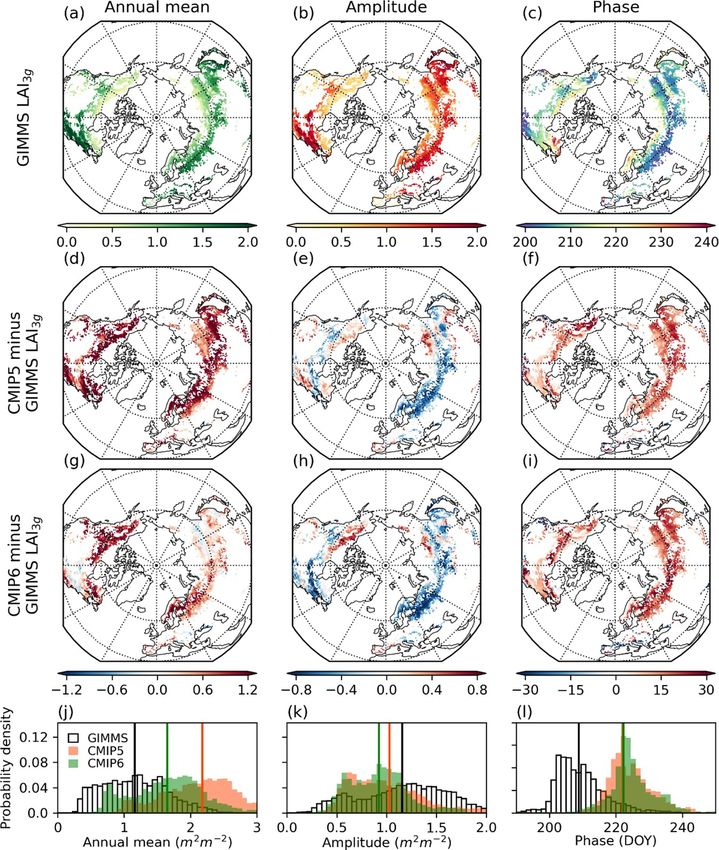
Figure 2. Mean distributions of LAI annual mean, amplitude, and phase from the GIMMS LAI3g (a)–(c), and the arithmetic
differences to those simulated by CMIP5 (d)–(f) and CMIP6 (g)–(i) models. Probability density functions of annual mean,
amplitude, and phase (j)–(l) of the GIMMS LAI3g and the CMIP5 and CMIP6 simulations, with their means (vertical lines) are
denoted in black, orange, and green, respectively.
60◦ N, and exceeded 30◦ in a few regions such as Figure 3 shows the mean patterns of SOS and EOS for
Alaska and Siberia, i.e. it was delayed by one month. 1982–2014, indicating the EOS is the primary cause
Notably, the observed SOS has advanced by a few days of the delayed seasonality. The spatial averages of the
over the past decades (Jeong et al 2011, Park et al SOSs were 152.3, 152.3, and 158.0 DOY in GIMMS
2018). However, this one-month delayed seasonality LAI3g , CMIP5, and CMIP6, respectively (figure 3(j)).
in boreal forests exhibits a significant difference in In the spatial pattern displayed by the CMIP5 mod-
vegetation seasonality, which can distort vegetation– els (figure 3(d)), the SOS difference was relatively
climate interactions during the growing season, and small, at less than 20 d in most of the high-latitude
may mislead future projections of the impact of cli- regions in Eurasia and North America. In contrast,
mate change on terrestrial ecosystems. in the CMIP6 models (figure 3(g)), the difference
This delayed LAI seasonality could be a result was larger than the results of the CMIP5, particu-
of the inaccurate representation of the growing sea- larly in certain high-latitude regions in Eurasia. The
son, i.e. a late SOS or EOS, in the CMIP6 model. ranges of the SOS differences from the 10th to 90th
8Environ. Res. Lett. 16 (2021) 034027 H Park and S Jeong
Figure 3. Mean distributions of SOS, EOS, and LOS for 1982–2014 from the GIMMS LAI3g (a)–(c) and the arithmetic differences
to those simulated by the CMIP5 (d)–(f) and CMIP6 (g)–(i) models. Probability density functions of SOS, EOS, and LOS (j)–(l)
of the GIMMS LAI3g and the CMIP5 and CMIP6 simulations, with their means (vertical lines) are denoted in black, orange, and
green, respectively.
percentile were −11.4 to 11.7 DOY in the CMIP5, Figures 3(e) and (h) clearly show the positive dif-
and −7.7 to 17.2 DOY in the CMIP6. This indic- ferences between EOS in CMIP5 and CMIP6, which
ates that the CMIP6 models tend to simulate later was the primary cause of the delayed LAI seasonal-
start in the growing season dates compared to the ity. The spatial averages of the EOS values were 260.8,
CMIP5 with regard to the mean distribution. The 282.7, and 279.1 DOY in the GIMMS LAI3g , CMIP5,
majority of the CMIP5 and CMIP6 models showed and CMIP6 outputs, respectively. Positive differences
relatively small biases in the mean values of SOS in the EOS of more than 20 d were most pronounced
that were less than 20 d, regardless of the latit- in high-latitude regions in both Eurasia and North
ude (supplementary figure 3(a) (available online at America, and exceeded 40 d in some regions in Alaska
stacks.iop.org/ERL/16/034027/mmedia)) and forest and Siberia. Europe and the southeastern part of
type (supplementary figure 4(a)). Hence, the differ- North America showed negative differences in EOS,
ence in SOS is not sufficient to fully explain the delay but their magnitudes and proportions were relatively
in LAI seasonality. minor compared to the clear positive biases shown
9Environ. Res. Lett. 16 (2021) 034027 H Park and S Jeong
Figure 4. (a) Taylor diagram representing pattern correlations (azimuthal angle) and normalized spatial standard deviations
(radial distance) of LAI annual mean (notated as ANN; circle), amplitude (AMP; plus), phase (PHS; cross), SOS (triangle), EOS
(square), and LOS (diamond) for the period of 1982–2014 in the CMIP5 (open) and CMIP6 (closed) models compared to the
GIMMS LAI3g over the northern temperate and boreal forests. The CMIP5 and CMIP6 ensembles are represented by open and
closed black markers, respectively. Pattern correlations of each seasonal indicator are denoted by numbers and colors for the (b)
CMIP5 and (c) CMIP6 ESMs.
at high latitudes. The 10th to 90th percentile ranges percentiles were 6.5 and 36.2 d, respectively. In the
of the EOS difference were 5.0–34.4 d in CMIP5 and case of CMIP6, the positive differences were relat-
−5.0–34.0 d in CMIP6. Although the positive differ- ively weak compared to those of CMIP5 in the high-
ences decreased slightly in CMIP6, both the CMIP latitude Eurasia region, with a narrow range shown
models showed similar severe delays in the EOS, by the 10th to 90th percentile (− 4.1–28.8 d). The
which led to the belated LAI seasonality simulated in results reveal that the simulated phenology shown by
the ESMs. This delay in autumn phenology, as shown the CMIP6 models tends to have a longer LOS res-
in the CMIP6 models, is consistent with the results of ulting from a later EOS, as compared to the GIMMS
previous studies on land surface models (Richardson LAI3g ; however, the bias to the satellite-derived LAI
et al 2012, Murray-Tortarolo et al 2013) and CMIP5 seasonality is decreased. The longer and later vegeta-
models (Anav et al 2013). Most CMIP5 and CMIP6 tion growing season contributes to the higher annual
models showed a positive bias in mean EOS that mean, weaker seasonal fluctuation, and delayed sea-
exceeded 20 d, especially at high latitudes (>50◦ N; sonality of LAI, as shown in figure 2. These large
supplementary figure 3(b)). In the case of forest type, biases in the mean LAI seasonality could be caused by
the belated EOS was distinct in deciduous needleleaf either a mean bias in a key climate variable (e.g. near-
forests, mixed forests, and woodlands (supplement- surface air temperature) or the misrepresentation
ary figure 4(b)), which are largely distributed at lat- of vegetation characteristics and processes (e.g. car-
itudes higher than 50◦ N (supplementary figure 2). bon allocation, phenology, or plant functional types).
This implies that both the CMIP5 and CMIP6 models However, the CMIP5 and CMIP6 did not show a sig-
do not appropriately describe the autumn senescence nificant mean bias in near-surface air temperature, in
of vegetation at high-latitude cold climate zones. contrast to LAI seasonality (supplementary figure 5).
The delay in the EOS resulted in a relatively longer This suggests that the positive biases in the mean SOS
LOS in both CMIP5 and CMIP6 models compared and EOS were largely derived from a misrepresenta-
to the GIMMS LAI3g , with an extension of more tion of deciduous forests in terms of vegetation prop-
than several pentads in certain high-latitude regions erties and processes.
(figures 3(f) and (i)). The spatial averages of the LOS In addition to the spatial patterns observed in
in the GIMMS LAI3g , CMIP5, and CMIP6 were 107.8, the CMIP5 and CMIP6 ensembles, we examined the
129.4, and 120.5 DOY, respectively. The LOS differ- LAI seasonality characteristics for each CMIP5 and
ences were mostly positive in the Northern Hemi- CMIP6 model. Figure 4 shows a Taylor diagram based
sphere in the CMIP5 outputs, and the 10th and 90th on the mean spatial patterns of seasonality indicators
10Environ. Res. Lett. 16 (2021) 034027 H Park and S Jeong
of phenological dates of the CMIP5 and CMIP6 mod- (f)), despite improvements in updated land surface
els. This diagram demonstrates that the majority of and phenological processes (tables 1 and 2). This
the models had pattern correlations lower than 0.8, clearly illustrates the difficulties in vegetation model-
indicating that ESMs cannot accurately represent the ing wherein changes in plant physiology and nutrient
spatial patterns of vegetation seasonality, even in his- dynamics can result in unintended consequences in
torical scenarios. The number of model outputs in a terms of vegetation seasonality.
relatively reliable range (with a pattern correlation of
>0.6, and a normalized standard deviation of >0.5 3.2. Responses of phenology to seasonal
and 60◦ N) dates is the near-surface air temperature for decidu-
indicates that the CMIP5 and CMIP6 models ten- ous forests distributed over the northern extratrop-
ded to show a better simulation performance over the ics (Jeong et al 2011). An accurate representation
lower-latitude regions (supplementary figures 6(a) of responses in phenology to seasonal temperature
and (d)) in terms of the mean spatial patterns. These change is closely connected to a long-term projec-
diagrams (figures 4(a), 6(a) and (d)) clearly illustrate tion of changes in terrestrial ecosystems under climate
that most of the ESMs faced difficulty in simulating change as well as its interactions with the Earth sys-
the mean characteristics in vegetation seasonality in tem. To briefly evaluate the phenological responses to
terms of both spatial variability and patterns. temperature in the CMIP5 and CMIP6 models, we
Figures 4(b) and (c) display colored tables con- compared the interannual sensitivities of the SOS and
taining pattern correlations of each indicator in the EOS to the corresponding seasonal temperature (T SOS
CMIP5 (upper panel) and CMIP6 (lower panel) and T EOS ) for each ESM in the deciduous forests
models to focus on whether each model could repro- (figure 5). The observation-based datasets (GIMMS
duce the mean spatial patterns of LAI seasonal- LAI3g and CRU TS) show a negative relationship
ity found in the GIMMS LAI3g . These panels show between SOS and T SOS , averaging −4.5 d K−1
that the ESMs simulated the SOS with the highest (figure 5(a)). Thus, higher spring temperatures were
correlations for most of the models. Most CMIP5 related to earlier SOS in deciduous forests. However,
and CMIP6 models showed correlations of higher the CMIP5 and CMIP6 ensembles showed a relatively
than 0.5, with improved values in CMIP6. In con- weak SOS sensitivity compared to the observation
trast, the results of the EOS were not in agreement (−2.2 and −2.6 d K−1 on average, respectively). In
with the GIMMS LAI3g in both the CMIP5 and particular, BCC-CSM1-1 and NorESM1-ME exhib-
CMIP6; most of the models showed low correla- ited the weakest sensitivities among the CMIP5 mod-
tions (less than 0.7). The exception was IPSL-CM6A- els (−1.0 and 0.0 d K−1 , respectively), but the newest
LR, which showed the best simulation performance versions indicated a stronger phenological response
of all phenological indicators, with a credible nor- to changes in near-surface air temperature (−2.3 and
malized standard deviation close to one and higher −2.5 d K−1 in BCC-CSM2-MR and NorESM2-LM,
pattern correlations than its previous version, IPSL- respectively). The sensitivity of SOS to T SOS tended
CM5A-MR. This improvement was largely due to bet- to be weaker in the CMIP5 and CMIP6 models, but
ter simulations of the EOS over the lower-latitude ESMs are able to simulate the advancement of SOS
regions (30–60◦ N; supplementary figures 6(b) and due to spring warming (figure 5(a)).
(c)). However, figures 4(b) and (c) also indicates In the case of the sensitivity of EOS to T EOS
that recent models are not always better for simu- (figure 5(b)), the observed sensitivity was positive
lating seasonality than previous versions. In the case (0.5 d K−1 ) on average, indicating that higher autumn
of the multi-model ensembles, the pattern correla- temperatures lead to a later EOS. The EOS sensit-
tions were lower in CMIP6 than in CMIP5 regard- ivities to T EOS tended to show a weaker magnitude
ing annual mean, amplitude, and EOS. This decrease than the SOS sensitivity to T SOS because the EOS
in correlation was distinct for the amplitude simu- is affected by not only autumn temperature but
lated in CESM2 and NorESM2-LM, which used the also environmental conditions such as insolation,
community land model 5 (CLM5) as the land surface leaf aging, and water availability (Liu et al 2016).
model (table 1). CESM2 and NorESM2-LM utilized The CMIP5 and CMIP6 ensembles showed a slightly
the same land models and had almost identical land larger magnitude of the EOS sensitivity (0.7 and
processes. As a result, they showed little difference 0.8 d K−1 on average, respectively), but the sensitivit-
in their partial correlations, despite differing evolu- ies of each model showed a large multi-model spread,
tions of seasonal meteorology. However, compared from −0.3 d K−1 of NorESM1-ME to 1.9 d K−1
to previous versions (CESM1-BCG and NorESM1- of CanESM2 in CMIP5, and from −0.6 d K−1 of
ME), the pattern correlations decreased significantly CESM2 to 2.9 d K−1 of MIROC-ES2L in CMIP6. Not-
for most of the seasonal indicators in both CESM2 ably, large proportions of deciduous forests in BCC-
and NorESM2-LM in both higher- and lower-latitude CSM1-1, CESM-BGC, and NorESM1-ME showed a
regions (supplementary figures 6(b), (c), (e) and weaker sensitivity compared to the other models, and
11Environ. Res. Lett. 16 (2021) 034027 H Park and S Jeong
Figure 5. Probability density functions of interannual sensitivities of (a) SOS to T SOS and (b) EOS to T EOS for the
observation-based datasets (GIMMS LAI3g with CRU TS; denoted as thick black line), CMIP5 ensemble (dashed black line),
CMIP6 ensemble (solid black line), and each CMIP5 (dashed line) and CMIP6 (solid line) model in deciduous forests over the
northern extratropics (>30◦ N) from 1982 to 2014. The means of probability density functions are indicated as vertical lines for
observation-based datasets, CMIP5, and CMIP6 ensembles. The ranges of the 10th to 90th percentiles (white box), 25th to 75th
percentiles (shaded box), medians (vertical bar), and means (closed circle) are also denoted.
the median sensitivities were close to zero (−0.1, and ∆T SOS (2005–2014 minus 1982–1991). The
0.1, and 0.0 d K−1 , respectively). In particular, in ellipse denotes the two-dimensional standard devi-
the CMIP6 models, CESM2 and NorESM2-LM con- ation of the ∆T SOS and ∆SOS distributions; if a
sistently displayed weak EOS sensitivity to autumn model displayed a change in temperature and pheno-
temperature, with medians of 0.0 d K−1 for both. logical dates identical to that of CRU TS and GIMMS
This irresponsive EOS in the two models seems to be LAI3g , its ellipse will be the same as the ellipse of the
related to a daylength-based trigger of growth offset observation. However, only a few models overlapped
in CLM4 and CLM5, and will be discussed in the sub- considerably with the observation ellipse of ∆SOS
sequent sections. and ∆T SOS (figure 6(a)). MIROC-ES2L had aver-
To determine whether the CMIP5 and CMIP6 ages of ∆SOS and ∆T SOS closest to the observation
models can represent recent changes in pheno- ellipse, and a few models (CESM1-BGC, MPI-ESM-
logical dates and temperature, we examined dif- MR, and MPI-ESM1-2-LR) showed similar averages
ferences in the mean distributions of SOS, EOS, regarding the ellipse of the observation. Most mod-
T SOS , and T EOS between the two periods of 1982– els tended to exaggerate ∆T SOS , that is, showing
1991 and 2005–2014 (i.e. ∆SOS, ∆EOS, ∆T SOS , stronger warming around the SOS than the obser-
and ∆T EOS ). Figure 6(a) shows the mean and vation, which resulted in the distant ellipses and
one-standard-deviation confidence ellipses of ∆SOS averages of models from the observation. In the
12Environ. Res. Lett. 16 (2021) 034027 H Park and S Jeong
Figure 6. Scatter plots of spatially averaged (a) ∆SOS with ∆T SOS (b) ∆EOS with ∆T EOS in the observation-based datasets
(GIMMS LAI3g with CRU TS; denoted as black squares), CMIP5 (triangles), and CMIP6 (circles) models in northern temperate
and boreal forests. The ellipses represent one-standard-deviation confidence regions of the distributions in the observation-based
datasets (thick black line), CMIP5 ensemble (dashed black line), CMIP6 ensembles (solid black line), and each model in CMIP5
(dashed lines) and CMIP6 (solid lines). Outliers exceeding two standard deviations were excluded from the analyses.
case of ∆EOS and ∆T EOS (figure 6(b)), five CMIP5 studies (Anav et al 2013, Murray-Tortarolo et al
models (BCC-CSM2-MR, CESM1-BGC, MIROC- 2013). Although there have been many improvements
ESM, MPI-ESM1-2, and NorESM1-ME), and three in land surface models since CMIP5 (tables 1 and 2),
CMIP6 models (CEMS2, MIROC-E2L, and MPI- this study reveals that even the latest CMIP6 mod-
ESM1-2-LR) exhibited means in the observation els do not sufficiently describe the LAI seasonality
ellipse. This represents the response of the EOS and phenological dates in terms of the mean distribu-
to autumn warming in the models with relatively tions (figure 4). Notably, the mean biases of EOS were
higher similarities to the observation, contrary to the more distinct than those of SOS, and this was com-
inaccurate representation of mean EOS distributions mon for the majority of the CMIP5 and CMIP6 ESMs.
(figures 3 and 4). Compared to the mean of the obser- This systematic delaying bias of EOS exceeded 20 d
vation, most models tended to have a lower ∆EOS on average at higher latitudes (>50◦ N; figure 3 and
but a higher ∆T EOS , similar to the higher ∆T SOS supplementary figure 3) and was also more distinct
shown in figure 6(a). Among the ESMs, MIROC- in deciduous needleleaf forests and woodlands, which
ES2L was shown to have the closest mean values to are mostly distributed over the cold climatic zones
the observation (figures 6(a) and (b)), which indic- (supplementary figures 2 and 4). The lower pattern
ates that MIROC-ES2L similarly simulated changes correlation at higher latitudes (supplementary figure
in seasonal temperature and involved phenological 6) implies that vegetation processes related to senes-
responses shown in CRU TS and GIMMS LAI3g for cence should be reexamined in boreal forests in order
both spring and autumn. to more accurately represent LAI seasonality.
The delayed autumn phenology shown in the
4. Discussion CMIP5 and CMIP6 models could have implications
regarding regional circulation and global climate
An accurate representation of LAI seasonality is through biases in energy balances as well as carbon
essential in the simulation of land–vegetation inter- fluxes. With regard to photosynthesis, delayed leaf
actions and long-term changes in climate (Richard- senescence is relatively less prominent in autumn
son et al 2012). Despite its importance, CMIP6 ESMs due to lower light availability (Jeong 2020, Zhang
tend to simulate the mean LAI seasonality with biases et al 2020), as compared to spring leaf emergence.
of larger annual means, weaker seasonal amplitude, However, delayed autumn phenology and a longer
and belated phases (figure 2) with delayed SOS and growing season in ESMs result in excessive mainten-
EOS (figure 3), as reported in previous CMIP5 model ance respiration and evapotranspiration with a lower
13Environ. Res. Lett. 16 (2021) 034027 H Park and S Jeong
surface albedo, which can lead to biases in surface in the physical processes of leaves (Arora and Boer
carbon fluxes, soil moisture, and energy partitioning 2005). For example, CLM uses a fixed length of
of net radiation into sensible and latent heat fluxes green-up periods (30 d), but the green-up duration
(Bonan 2008, Piao et al 2020a). Considering the varies with temperature (Park et al 2015, 2020). The
importance of interactions between vegetation and present land surface model is not sufficiently accurate
climate, the inaccurate representation of EOS in the because of knowledge gaps, particularly for autumn
northern extratropics could lead to significant biases leaf senescence (Jeong 2020). Another example is
in seasonal climate patterns on both regional and the sensitivity of the EOS to temperature. EOS is
global scales (Richardson et al 2012). In full-couple influenced by a variety of complex factors such as
carbon cycle simulations, biases in spring or autumn daytime and nighttime temperature, precipitation,
phenology lead to biases in surface carbon fluxes and photoperiod, and leaf aging (Jeong 2020, Keenan and
atmospheric carbon concentration, which can accu- Richardson 2015, Liu et al 2016, Chen et al 2020).
mulate over time and result in large uncertainties However, as mentioned above, CLM determines the
regarding long-term climate predictions (Richardson start of the leaf senescence stage of seasonal decidu-
et al 2012, Friedlingstein et al 2014). For climate sim- ous forests solely by using daylength. As a result, the
ulations that do not include the prognostic carbon EOS sensitivity to T EOS was close to zero for all the
cycle, biases in LAI seasonality can lead to differing CLM-based ESMs in CMIP5 and CMIP6 (CESM1-
evolutions of seasonal meteorology and further long- BGC, CESM2, NorESM1-ME, and NorESM2-LM in
term climate issues through the distortion of surface figure 5(b)). In the case of the CTEM of BCC-CSM2-
hydrology and energy balances. The results of this MR and CanESMs, the start of senescence is triggered
study imply that phenology schemes, particularly for by consecutive days of net carbon loss due to unfavor-
autumn phenology, need to be improved in order to able weather conditions, such as shorter day lengths,
obtain a more accurate representation of vegetation colder temperatures, and drier soil moisture, based
seasonality and predictions for long-term climate on a carbon benefit approach (Arora and Boer 2005).
change. In contrast, ORCHIDEE of IPSL-CM6A-LR utilizes
The LAI seasonality and phenology in the land leaf age, along with the temperature threshold, to
surface models are comprehensive and consequential parameterize litter fall and senescence (Krinner et al
phenomena related to various terrestrial ecosystem 2005). Although the CTEM and ORCHIDEE ten-
processes (e.g. start or end of leaf carbon allocation, ded to exaggerate the EOS sensitivity to temperature
carbon allocation fluxes, and PFTs representation). more than that shown in the GIMMS LAI3g and CRU
Therefore, they cannot be simulated realistically TS, it is suggested that the CLM4 and CLM5 should
unless all the ecosystem processes are in tune. For include other variables to describe the EOS responses
example, in the case of seasonal deciduous forests to temperature variation.
in CLM, the spring green-up stage is initiated when The responses of spring and autumn phenology
the accumulated soil temperature exceeds a threshold to seasonal temperature variation is another notable
that is determined by the annual mean 2 m air tem- issue still possessed by state-of-the-art ESMs as well as
perature of each grid point (Lawrence et al 2011). the mean biases. Both CMIP5 and CMIP6 ESMs tend
After this leaf onset, stored carbon transfers to the to underestimate the SOS sensitivities compared to
leaf during a fixed period of 30 d, which results in GIMMS LAI3g (figure 5(a)). This suggests that even if
an increase in LAI depending on the specific leaf ESMs project a future warming pattern of spring tem-
area of the PFTs. In autumn, senescence is triggered perature with high accuracy, the weaker SOS sensitiv-
when the day length is shorter than a critical value, ities in the ESMs will result in an underestimation of
and the leaves lose their carbon over 15 d (i.e. the the SOS change due to warming and its interactions,
LAI decreases). Changes in photosynthesis and res- for example, transpiration and cloudiness (Chen et al
piration due to meteorological conditions and nutri- 2016, Ma et al 2016). Therefore, the phenological
ent dynamics can influence the phenological dates sensitivity of SOS and EOS should be improved to
because LAI depends on leaf carbon content. Any achieve better projection of terrestrial ecosystems and
biases in either meteorology, PFTs, or the senescence their role in climate systems in the future.
threshold can result in biased LAI seasonality, as Seasonal warming is another notably import-
shown in this study. Murray-Tortarolo et al (2013) ant factor that can have a significant influence on
reported positive biases in the phenological dates of phenology simulations (figure 6). Many of the ESMs
land surface model simulations based on imposed showed a stronger warming in spring and autumn
PFTs and meteorological forcing. This implies that than CRU TS. This stronger warming in the mod-
the belated biases in the LAI seasonality, especially in els can lead to earlier SOS and later EOS than those
the EOS, are likely to result from vegetation schemes in the GIMMS LAI3g , even in the case where the
rather than PFTs and model meteorology. land surface models are ideal for describing changes
Our understanding remains insufficient to in phenology. Therefore, realistic predictions of sea-
describe vegetation phenology and its relationships sonal temperature changes are a prerequisite for
with environmental conditions due to complexities accurate representation of the response of vegetation
14Environ. Res. Lett. 16 (2021) 034027 H Park and S Jeong
seasonality to climate change. For example, CESM2 (Bonan 2008). For example, delayed LAI seasonal-
and NorESM2-LM are based on the same land sur- ity over high latitudes can lead to a high temper-
face model (CLM5), and their mean sensitivities of ature bias by lowering the surface albedo, and can
SOS to temperature are almost the same (−2.6 and amplify the biases in autumn phenology by exagger-
−2.5 d K−1 , respectively). However, there is a large ating autumn temperature. Therefore, the sensitiv-
difference in ∆SOS and ∆T SOS because of the differ- ities of phenological dates to seasonal temperature
ent spring warming patterns between the two mod- (figure 5) could be affected by the interactions and
els (figure 6). This demonstrates the importance of feedback processes between the vegetation seasonal-
accurate projections of future climate change to fore- ity and environmental conditions. Here, we aimed
see the changes in spring and autumn phenology. to illustrate the overall aspects of the CMIP6 LAI on
In this study, we focused on the overall evalu- the basis of monthly output, which is not a thorough
ation of LAI seasonality and its responses to seasonal investigation of the two-way consequence because of
temperature in CMIP6 in comparison with the pre- the misrepresentation of LAI seasonality. In future
vious CMIP5 and GIMMS LAI3g . However, it should studies, a daily examination of LAI and temperature
be noted that our results could be affected by uncer- is required to clarify the consequences of delayed LAI
tainties in either snow contamination of the satel- seasonality and its feedbacks.
lite data or differences in spatiotemporal resolutions The vegetation fraction is an important factor that
between models. The satellite-retrieved LAI dataset affects land-surface albedo and evapotranspiration
is a valuable tool for evaluating LAI seasonality in (Brovkin et al 2013), which in turn influences LAI
ESMs over a wide range, but its potential uncer- seasonality in the ESMs. The CMIP6 ESMs require
tainties such as snow contamination in high-latitude a standard land-use scenario, land use harmoniza-
regions, should be discussed. In this study, we utilized tion 2 (LUH2), to facilitate intercomparison analyses
the GIMMS LAI3g based on a 15 d maximum com- of the ESMs (Eyring et al 2016, Hurtt et al 2020,
posite and logistic fitting methods, to minimize the Ma et al 2020). In spite of the same land-use scen-
uncertainties in LAI seasonality related to snow. The ario, the implementation of LUH2 could lead to a
maximum composite and logistic fitting were effect- discrepancy in vegetation or forest fractions due to
ive methods for reducing non-vegetative influences, different translation rules, or inconsistent PFTs of
but the non-vegetative influence of snow could not be each ESM (table 2). Under the same land-use for-
completely removed from the analysis. Considering cing, the discrepancy in forest fractions among ESMs
that uncoupled land model simulations have shown a is likely to be minor compared to other uncertainties.
delay in LAI seasonality similar to this study (Murray- Considering the importance of vegetation fractions,
Tortarolo et al 2013) and more realistic snow season- however, the discrepancy and its consequent influ-
ality in CMIP6 models (Mudryk et al 2020), the influ- ences need to be clarified in intercomparison studies
ence of snow cover could be relatively minor com- focusing on vegetation fraction and PFTs between the
pared to the large biases in LAI seasonality. ESMs.
Another uncertainty can arise from the differ-
ences between the maximum-composite satellite LAI
and the monthly averaged LAI from the CMIP mod- 5. Conclusion
els. GIMMS LAI3g is based on the 15 d maximum
composite to minimize potential uncertainties, which This study reveals that CMIP6 ESMs show a large bias
is not identical to monthly averaging and can cre- in LAI seasonality and phenological dates with regard
ate a bias between the satellite and modeled LAI. to the mean distributions and responses to temperat-
This methodological difference can partly contrib- ure in deciduous forests over the northern extratrop-
ute to the delayed biases of autumn phenology, but ics, which is similar to the CMIP5 ESMs. These veget-
cannot fully explain the EOS differences between the ation seasonality biases can result in inaccurate rep-
GIMMS LAI3g and ESMs that exceed 40 d. Neverthe- resentations of vegetation–climate interactions such
less, applying the maximum composite to daily LAI as surface energy balance, hydrological processes, and
output from the models will be a way to ensure con- carbon fluxes. Our findings highlight that decidu-
sistency between the model output and satellite data ous phenology, particularly leaf senescence, should be
for precise analyses. The harmonization of different improved for a more accurate depiction of terrestrial
spatial resolutions among CRU TS, GIMMS LAI3g , ecosystems and their interactions with the Earth
and ESMs (table 1), or the limited number of years system.
(33 years from 1982 to 2014), could also have caused
uncertainties in our analyses.
This study assumed that seasonal temperat- Data availability statement
ure exerts a one-way influence on LAI seasonality,
while LAI exerts an influence on temperature by The data that support the findings of this study are
modulating evapotranspiration and surface albedo available upon reasonable request from the authors.
15Environ. Res. Lett. 16 (2021) 034027 H Park and S Jeong
Acknowledgments Dufresne J L et al 2013 Climate change projections using the
IPSL-CM5 Earth system model: from CMIP3 to CMIP5
Clim. Dyn. 40 2123–65
We thank two anonymous reviewers for their con-
Eyring V, Bony S, Meehl G A, Senior C A, Stevens B, Stouffer R J
structive comments, which helped us to improve and Taylor K E 2016 Overview of the Coupled Model
the quality of this study. This work was suppor- Intercomparison Project Phase 6 (CMIP6) experimental
ted by grants from the National Research Found- design and organization Geosci. Model Dev.
9 1937–58
ation of Korea (NRF) Korea (MSIT) (MSIT; Nos.
Friedlingstein P, Meinshausen M, Arora V K, Jones C D, Anav A,
2019R1C1C1004826 and 2019R1A2C3002868). We Liddicoat S K and Knutti R 2014 Uncertainties in CMIP5
acknowledge the World Climate Research Pro- climate projections due to carbon cycle feedbacks J. Clim.
gramme, which, through its Working Group on 27 511–26
Garonna I, De Jong R, Stöckli R, Schmid B, Schenkel D, Schimel D
Coupled Modelling, coordinated and promoted
and Schaepman M E 2018 Shifting relative importance of
CMIP6. We thank the climate modeling groups for climatic constraints on land surface phenology Environ. Res.
producing and making available their model output, Lett. 13 024025
the Earth System Grid Federation (ESGF) for archiv- Giorgetta M A et al 2013 Climate and carbon cycle changes from
1850 to 2100 in MPI-ESM simulations for the Coupled
ing the data and providing access, and the multiple
Model Intercomparison Project phase 5 J. Adv. Model. Earth
funding agencies who support CMIP6 and ESGF. Syst. 5 572–97
Hajima T et al 2020 Description of the MIROC-ES2L Earth
system model and evaluation of its climate–biogeochemical
processes and feedbacks Geosci. Model Dev.
ORCID iDs 13 2197–244
Hansen M C, Sohlberg R, Defries R S and Townshend J R G 2000
Hoonyoung Park https://orcid.org/0000-0002- Global land cover classification at 1 km spatial resolution
using a classification tree approach Int. J. Remote Sens. 21
7856-5218 1331–64
Sujong Jeong https://orcid.org/0000-0003-4586- Harris I, Osborn T J, Jones P and Lister D 2020 Version 4 of the
4534 CRU TS monthly high-resolution gridded multivariate
climate dataset Sci. Data 7 1–18
Hurrell J W et al 2013 The community Earth system model: a
References framework for collaborative research Bull. Am. Meteorol.
Soc. 94 1339–60
Anav A, Murray-Tortarolo G, Friedlingstein P, Sitch S, Piao S and Hurtt G C et al 2020 Harmonization of global land use change
Zhu Z 2013 Evaluation of land surface models in and management for the period 850–2100 (LUH2) for
reproducing satellite derived leaf area index over the CMIP6 Geosci. Model Dev. 13 5425–64
high-latitude Northern Hemisphere. Part II: Earth system Ito A and Oikawa T 2002 A simulation model of the carbon cycle
models Remote Sens. 5 3637–61 in land ecosystems (Sim-CYCLE): a description based on
Arora V K et al 2020 Carbon-concentration and carbon-climate dry-matter production theory and plot-scale validation Ecol.
feedbacks in CMIP6 models and their comparison to Modelling 151 143–76
CMIP5 models Biogeosciences 17 4173–222 Iversen T et al 2013 The Norwegian Earth system model,
Arora V K and Boer G J 2005 A parameterization of leaf NorESM1-M—part 2: climate response and scenario
phenology for the terrestrial ecosystem component of projections Geosci. Model Dev. 6 389–415
climate models Glob. Change Biol. 11 39–59 Jeong S J, Ho C H, Gim H J and Brown M E 2011 Phenology shifts
Arora V K, Scinocca J F, Boer G J, Christian J R, Denman K L, at start vs. end of growing season in temperate vegetation
Flato G M, Kharin V V, Lee W G and Merryfield W J 2011 over the Northern Hemisphere for the period 1982–2008
Carbon emission limits required to satisfy future Glob. Change Biol. 17 2385–99
representative concentration pathways of greenhouse gases Jeong S J, Ho C H, Kim K Y and Jeong J H 2009 Reduction of
Geophys. Res. Lett. 38 L05805 spring warming over East Asia associated with vegetation
Bentsen M et al 2013 The Norwegian Earth system model, feedback Geophys. Res. Lett. 36 L18705
NorESM1-M—part 1: description and basic evaluation of Jeong S 2020 Autumn greening in a warming climate Nat. Clim.
the physical climate Geosci. Model Dev. 6 687–720 Change 10 712–13
Bonan G B 2008 Forests and climate change: forcings, feedbacks, Jeong S and Park H 2020 Toward a comprehensive understanding
and the climate benefits of forests Science 320 1444–9 of global vegetation CO2 assimilation from space Glob.
Boucher O et al 2020 Presentation and evaluation of the Change Biol. 1–3
IPSL-CM6A-LR climate model J. Adv. Model. Earth Syst. 12 Jinjun J 1995 A climate-vegetation interaction model: simulating
1–52 physical and biological processes at the surface J. Biogeogr.
Brovkin V, Boysen L, Raddatz T, Gayler V, Loew A and Claussen 22 445–51
M 2013 Evaluation of vegetation cover and land-surface Keenan T F and Richardson A D 2015 The timing of autumn
albedo in MPI-ESM CMIP5 simulations J. Adv. Model. Earth senescence is affected by the timing of spring phenology:
Syst. 5 48–57 implications for predictive models Glob. Change Biol.
Chen L, Hänninen H, Rossi S, Smith N G, Pau S, Liu Z, Feng G, 21 2634–41
Gao J and Liu J 2020 Leaf senescence exhibits stronger Knorr W 2000 Annual and interannual CO2 exchanges of the
climatic responses during warm than during cold autumns terrestrial biosphere: process-based simulations and
Nat. Clim. Change 10 777–80 uncertainties Glob. Ecol. Biogeogr. 9 225–52
Chen M, Melaas E K, Gray J M, Friedl M A and Richardson A D Krinner G, Viovy N, De Noblet-ducoudré N, Ogée J, Polcher J,
2016 A new seasonal-deciduous spring phenology submodel Friedlingstein P, Ciais P, Sitch S and Prentice I C 2005 A
in the community land model 4.5: impacts on carbon and dynamic global vegetation model for studies of the coupled
water cycling under future climate scenarios Glob. Change atmosphere-biosphere system Glob. Biogeochem. Cycles
Biol. 22 3675–88 19 1–33
Danabasoglu G et al 2020 The community earth system model Lawrence D M et al 2011 Parameterization improvements and
version 2 (CESM2) J. Adv. Model. Earth Syst. functional and structural advances in version 4 of the
12 1–35 community land model J. Adv. Model. Earth Syst. 3 M03001
16You can also read