NOVEL TILE SEGMENTATION SCHEME FOR OMNIDIRECTIONAL VIDEO

Page created by Sylvia Garcia
 
CONTINUE READING
NOVEL TILE SEGMENTATION SCHEME FOR OMNIDIRECTIONAL VIDEO

                                                                Jisheng Li, Ziyu Wen, Sihan Li, Yikai Zhao, Bichuan Guo, Jiangtao Wen

                                                                                                    Tsinghua University
                                                                                                   Beijing, 100084, China

                                                                     ABSTRACT
arXiv:2103.05858v1 [cs.CV] 10 Mar 2021

                                              Regular omnidirectional video encoding technics use map pro-
                                         jection to flatten a scene from a spherical shape into one or several
                                         2D shapes. Common projection methods including equirectangular
                                         and cubic projection have varying levels of interpolation that create a
                                         large number of non-information-carrying pixels that lead to wasted
                                         bitrate. In this paper, we propose a tile based omnidirectional video
                                         segmentation scheme which can save up to 28% of pixel area and
                                         20% of BD-rate averagely compared to the traditional equirectangu-                                                      (b) Cubic (190%)
                                                                                                                      (a) Equirectangular (157%)
                                         lar projection based approach.
                                             Index Terms— Omnidirectional video, tile segmentation

                                                                1. INTRODUCTION

                                         The ever wider application of virtual reality (VR) requires that omni-
                                         directional video for consumption on VR devices be efficiently cap-
                                         tured, encoded and transmitted.
                                              Various types of equipment for recording omnidirectional video                (c) Tile (123%)                  (d) Proposed Tile (113%)
                                         has already been developed. Most of these capturing equipments
                                         use two fish-eye cameras or multiple wide angle cameras to cap-
                                                                                                                    Fig. 1. Comparison of map projections under same minimum sample
                                         ture the scene and then stitch frames from these cameras together.
                                                                                                                    density on the sphere (with percentage of original sphere area in the
                                         In this process, an omnidirectional picture well represented using a
                                                                                                                    brackets). (c) A tile segmentation scheme with equal division on
                                         spherical surface is created, and then mapped into a flat plane for
                                                                                                                    latitude; (d) Our proposed 5-tiles scheme
                                         subsequent encoding and then transmitted. A number of mapping
                                         methods from the spherical to flat surfaces have been proposed, such
                                         as the technique in [1] [2] [3], with various distortions created during
                                         the process [4].                                                           areas in the north and south poles of the sphere are stretched more
                                              In this paper, we propose a tile-based segmentation and pro-          severely than areas near the equator, overall, a net increase of 57%
                                         jection scheme. It attempts to create an approximate equal-area            of the original sphere area was introduced wastefully, leading to a
                                         mapping and projection with compression-friendly shapes with less          resultant increase in bitrate. Furthermore, due to the distortions in-
                                         wasteful pixels. Our scheme can save up to 28% of pixel area com-          troduced by the stretching, especially near the two poles, predictive
                                         pare to equirectangular projection and 40% of pixel area compare to        coding tools in video encoders fail more easily, causing further re-
                                         cubic [5] projection at the same minimum sampling density in the           duction in coding efficiency.
                                         original spherical surface.                                                     In [5], Ng et al. proposed a method to project a sphere onto a
                                              The paper is organized as follows: In section 2, we review re-        cube, referred as cubic projection subsequently. Although the dis-
                                         lated work and the quality metric. Section 3 describes the proposed        tortion introduced by projection is mitigated in cubic projection, the
                                         tile segmentation scheme in details. Experimental results are shown        total area of the 6 sides has to be 190% of the original sphere area
                                         in section 4 while section 5 is the conclusion.                            so that the central of each surface has enough sample density, as is
                                                                                                                    shown in Fig.1. Later in [9], Fu et al. proposed a rhombic dodecahe-
                                                                2. RELATED WORK                                     dron map projection scheme, which divided a sphere into 12 rhombs
                                                                                                                    then reshape to squares and rearrange into a rectangular.
                                         Many early techniques for capturing omnidirectional video [6] [7]               In [10], Yu et al. divided the video vertically into tiles and re-
                                         used a camera and a parabolic mirror. The camera captures images           sized the tiles according to the latitudes or user preferences (e.g. ar-
                                         reflected by the parabolic mirror, with the vertical field of view lim-    eas near the poles might be less likely to be requested by the viewer).
                                         ited in 90◦ .                                                              Even though this scheme solved many of the issues caused by stretch
                                              Lately, higher quality omnidirectional video are captured with        related distortions and increase in the total number of pixels after
                                         multiple high definition cameras with the captured frames stitched         mapping, it did not fully address the issue of preserving effective-
                                         [8]. When projecting the image to a flat 2D plane, equirectangular         ness of predictive coding tools in video encoders.
                                         projection was widely used. Despite of its ease of use, because the             There are relatively few studies on methods for evaluating video
3.1. Area comparison
                                                                          The total area of each hemisphere’s tiles can be describe as:
                                                                                                                           n
                                                                                                                           X
                                                                                     Shemisphere = Spole +                       2πr2 cos θi−1 (θi − θi−1 ) .        (1)
                                                                                                                           i=1

                                                                                                                     π( π2 − θp )2 r2
                                                                                                                 
                                                                                                                                         , Circle Pole
                                                                                                       Spole =                                         .             (2)
                                                                                                                     4( π2 − θp )2 r2   , Square Pole
                  (a) A tile segmentation example                         where θ1 , θ2 ...θn are the latitude (in rad) of the borders, e.g. for
                                                                          north hemisphere θ1 , θ2 ...θn ∈ (0, π2 ) and θ1 < θ2 < ... < θn =
                                                                          θp . θ0 = 0 corresponds to the latitude of the equator, while θp is the
                                                                          latitude of the outer edge of the pole areas which is actually the same
                                                                          with θn . After n cuts at each hemisphere, the sphere is projected and
                                                                          divided into (2n + 1) tiles, with one big tile across the equator.
                                                                               In the tile segmentation method proposed in Yu’s work[10], the
                                                                          area of pole under same minimum sample density is
                                                                                                                                  π
                                                                                                          Spole,Yu = 2πr2 (         − θp ) cos θp .                  (3)
               (b) A rearrangement layout for 3-tiles                                                                             2
                                                                          which is always larger than Eq.2 .
                                                                               The best segmentation scheme can be found by minimizing the
                                                                          total area given a number of the tiles n:

                                                                                              Θn = {θ1 , ..., θn } =             arg min       Shemisphere .         (4)
                                                                                                                            0
1.25
                                                                      Overlap 0.7%         Table 1. Optimization results on specified tiles number and overlap
                                                                      Overlap 0.5%
                                                                      Overlap 0.3%         percentage (in degrees)
                                                                      Overlap 0%
                   1.2                                                                           Scheme        0% overlap 0.3% overlap 0.5% overlap
                                                                                                  3-tiles
                                                                                                               θ1 =32.70◦     θ1 =32.97◦       θ1 =33.15◦
                                                                                               (Circle pole)
                                                                                                               θ1 =25.34◦     θ1 =26.08◦       θ1 =26.58◦
  Area (/4:r2 )

                  1.15                                                                            5-tiles
                                                                                               (Circle pole)   θ2 =38.22◦     θ2 =38.81◦       θ2 =39.21◦
                                                                                                  3-tiles
                                                                                                               θ1 =45.00◦     θ1 =45.27◦       θ1 =45.45◦
                   1.1                                                                        (Square pole)
                                                                                                  5-tiles      θ1 =35.07◦     θ1 =35.81◦       θ1 =36.30◦
                                                                                                                         ◦                ◦
                                                                                              (Square pole) θ2 =53.17         θ2 =53.77        θ2 =54.18◦
                  1.05

                                                                                                            4. EXPERIMENTAL RESULTS
                    1
                         0        2            4         6        8           10
                                            n (Cuts per hemisphere)                        4.1. Non-overlapping RD performance

Fig. 4. Total area comparison of different tile number and overlap                         The RD performance experiments were conducted with the widely
(Square poles)                                                                             used open source HEVC encoder x265[12] on its default settings.
                                                                                           The test sequences are from two datasets. The first 10 sequences in
                                                                                           Table 2 and Table 3 are 9K images from SUN360 database[13], and
3.2. Overlapping                                                                           the last two sequences are 4K video clips generously provided by
                                                                                           LETINVR.
When a tiled video is encoded at a low bitrate, border artifacts exist                          The QPs used for computing the BD-rate are 22, 27, 32, 37.
between tile boundaries. A common approach to this issue is to set                         For the quality metric, we use the S-PSNR and L-PSNR as in [11]
overlapping areas between tiles.                                                           and introduced in Section 2. The S-PSNR weights all position on
    Introducing overlaps will increase the total area. Hence the op-                       the sphere equally while the L-PSNR weights positions according
timization problem in (4) becomes:                                                         to its latitude access frequency. In our experiments, we measured
                                                                                           both metrics and we used both S-PSNR and L-PSNR in the BD-Rate
                                                                      σπ
                     Shemisphere (σ) = Spole (σ) + 2πr2 (θ1 +            )                 calculations.
                                                                       2                        As the test sequences are all in equirectangular projection for-
                                      n                                              (5)
                                      X                                                    mat as ground truth, we down-sampled the sequences in the experi-
                                 +          2πr2 cos θi−1 (θi − θi−1 + σπ) .
                                                                                           ments so that the ground truth has always higher sample density. For
                                      i=2
                                                                                           example, the SUN360 experiments were conducted at 4552x2276
                                π                  σπ 2 2                                 while the inputs are at 9104x4552 equirectangular. When calculat-
                                π( 2 − θp +          2
                                                       ) r     , Circle Pole
                   Spole (σ) =                      σπ 2 2                   .       (6)   ing S-PSNR and L-PSNR, decoded sequences were mapped back to
                                4( π2 − θp +           ) r    , Square Pole
                                                     2                                     equirectangular with the original input resolution. Bilinear interpo-
                                                                                           lation was used in above steps.
                         Θn,σ = {θ1 , ..., θn }                                                 The experiment results are shown in Fig.5, Table 2 and Table
                              =          arg min          Shemisphere (σ) .          (7)   3, including proposed 3-tiles scheme (P3), proposed 5-tiles scheme
                                 σπ
38                                                                                               38
                                 Equirectangular                                                                                  Equirectangular
                                 3-tiles                                                                                          3-tiles
                                 5-tiles                                                                              37          5-tiles
                     37          Cubic                                                                                            Cubic
                                 Yu's 3-tiles                                                                                     Yu's 3-tiles
                                 Yu's 5-tiles                                                                                     Yu's 5-tiles
                                                                                                                      36
                     36

                                                                                                                      35
       S-PSNR (dB)

                                                                                                        L-PSNR (dB)
                     35
                                                                                                                      34
                     34
                                                                                                                      33

                     33
                                                                                                                      32

                     32                                                                                               31

                     31                                                                                               30
                          0          20            40          60           80   100                                       0          20            40          60           80   100
                                            bitrate (Mbps, 25fps as all intra)                                                               bitrate (Mbps, 25fps as all intra)

                              (a) RD curve of Seq. 1 using S-PSNR                                                              (b) RD curve of Seq. 1 using L-PSNR

                                                           Fig. 5. RD curves of two sequences with S-PSNR and L-PSNR metric.

   Table 2. BD-Rate of proposed method using S-PSNR
  Seq.     P3       P5        CP        Y3        Y5
     1 -11.6%      -9.8%     -4.6%     -5.5%     -4.5%
     2 -13.1% -13.4%         -9.2% -10.2% -10.4%
     3 -12.5% -11.8% -12.2%            -7.4%     -7.5%
     4 -10.6% -10.0%         -7.3%     -6.8%     -7.2%
     5 -15.2% -16.4% -10.3% -12.3% -12.9%
     6    -8.0% -14.7%       -3.1%     -7.5%     -7.7%
     7 -12.9% -13.1%         -8.2% -10.3% -11.0%
     8    -8.4%    -7.0%     -1.4%     -4.5%     -3.9%
     9    -1.4%     1.0%      1.2%      0.9%      2.8%
    10 -13.7% -13.4%         -9.6%     -9.7% -10.9%
    11 -16.8% -18.6%         -0.4% -11.3% -14.6%
    12 -22.5% -23.9%         -7.8% -13.6% -17.5%
  Avg. -12.2% -12.6%         -6.1%     -8.2%     -8.8%

   Table 3. BD-Rate of proposed method using L-PSNR
  Seq.     P3       P5        CP        Y3        Y5
     1 -18.5% -17.5% -11.8% -10.0% -10.3%
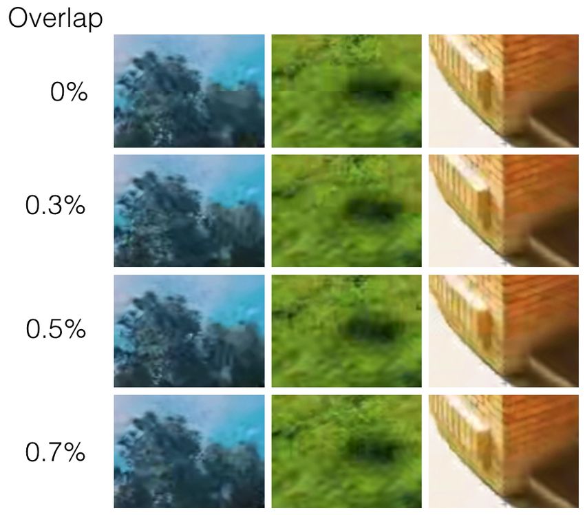
     2 -17.9% -18.3% -12.3% -13.6% -14.7%                                                     Fig. 6. Comparison on the border of tile with 0%, 0.3%, 0.5% and
     3 -19.7% -19.2% -18.8% -12.2% -13.2%                                                     0.7% overlap from top to bottom, QP = 37.
     4 -19.8% -19.3% -17.3% -11.3% -12.9%
     5 -24.6% -25.0% -22.1% -16.2% -17.8%
     6 -20.4% -19.9% -18.7% -12.7% -14.4%
     7 -27.6% -27.0% -24.7% -16.9% -19.5%                                                                                                  5. CONCLUSION
     8 -16.4% -15.5%         -9.7%     -8.5%     -9.0%
     9 -10.6%      -8.3%     -7.4%     -4.2%     -3.6%                                        In this paper, we proposed a tile segmentation scheme for omnidi-
    10 -21.7% -21.3% -10.0% -13.8% -16.2%                                                     rectional video encoding, which has less pixel wastage and more le-
    11 -22.5% -23.9%         -7.8% -24.1% -23.9%                                              gitimate mapping method. Experimental results show the proposed
    12 -21.9% -21.0%         -5.0% -11.9% -13.1%                                              scheme can save up to 28% of pixel area and 20% BD-rate averagely
  Avg. -20.1% -19.7% -14.6% -13.0% -14.1%                                                     compare to traditional equirectangular projection.
                                                                                                   Future work includes optimization on segmentation scheme tar-
Table 4. BD-rate result of 0.5% overlap compare to 0% overlap                                 geting on region of interest (ROI) application, as well as optimiza-
                       S-PSNR          L-PSNR                                                 tions on temporal and spacial random access.
           Seq.
                     P3       P5      P3     P5
               1 0.8% 1.2% 0.9% 1.4%
               2 1.4% 0.4% 1.6% 0.4%                                                                                                       6. REFERENCES
               3 0.9% 2.3% 0.8% 2.2%
               4 1.0% 1.4% 1.1% 1.6%                                                           [1] John P Snyder, Flattening the earth: two thousand years of
               5 1.0% 1.9% 1.1% 1.9%                                                               map projections, University of Chicago Press, 1997.
               6 1.1% 2.3% 1.3% 2.6%
                                                                                               [2] Shenchang Eric Chen, “Quicktime vr: An image-based ap-
           Avg. 1.0% 1.6% 1.1% 1.7%                                                                proach to virtual environment navigation,” in Proceedings of
the 22nd annual conference on Computer graphics and inter-
     active techniques. ACM, 1995, pp. 29–38.
 [3] Richard Szeliski and Heung-Yeung Shum, “Creating full view
     panoramic image mosaics and environment maps,” in Pro-
     ceedings of the 24th annual conference on Computer graphics
     and interactive techniques. ACM Press/Addison-Wesley Pub-
     lishing Co., 1997, pp. 251–258.
 [4] Denis Zorin and Alan H Barr, “Correction of geometric percep-
     tual distortions in pictures,” in Proceedings of the 22nd annual
     conference on Computer graphics and interactive techniques.
     ACM, 1995, pp. 257–264.
 [5] King-To Ng, Shing-Chow Chan, and Heung-Yeung Shum,
     “Data compression and transmission aspects of panoramic
     videos,” Circuits and Systems for Video Technology, IEEE
     Transactions on, vol. 15, no. 1, pp. 82–95, 2005.
 [6] Ivana Tošić and Pascal Frossard, “Low bit-rate compression of
     omnidirectional images,” in Picture Coding Symposium, 2009.
     PCS 2009. IEEE, 2009, pp. 1–4.
 [7] Ingo Bauermann, Matthias Mielke, and Eckehard Steinbach,
     “H. 264 based coding of omnidirectional video,” in Computer
     Vision and Graphics, pp. 209–215. Springer, 2006.
 [8] Patrice Rondao Alface, Jean-François Macq, and Nico Verz-
     ijp, “Interactive omnidirectional video delivery: A bandwidth-
     effective approach,” Bell Labs Technical Journal, vol. 16, no.
     4, pp. 135–147, 2012.
 [9] Chi-Wing Fu, Liang Wan, Tien-Tsin Wong, and Chi-Sing Le-
     ung, “The rhombic dodecahedron map: An efficient scheme
     for encoding panoramic video,” Multimedia, IEEE Transac-
     tions on, vol. 11, no. 4, pp. 634–644, 2009.
[10] Matt Yu, Haricharan Lakshman, and Bernd Girod, “Content
     adaptive representations of omnidirectional videos for cine-
     matic virtual reality,” in Proceedings of the 3rd International
     Workshop on Immersive Media Experiences. ACM, 2015, pp.
     1–6.
[11] Matt Yu, Haricharan Lakshman, and Bernd Girod, “A frame-
     work to evaluate omnidirectional video coding schemes,” in
     Mixed and Augmented Reality (ISMAR), 2015 IEEE Interna-
     tional Symposium on. IEEE, 2015, pp. 31–36.
[12] “x265,” http://x265.org.
[13] Jianxiong Xiao, Krista A Ehinger, Aude Oliva, and Anto-
     nio Torralba, “Recognizing scene viewpoint using panoramic
     place representation,” in Computer Vision and Pattern Recog-
     nition (CVPR), 2012 IEEE Conference on. IEEE, 2012, pp.
     2695–2702.
You can also read