Operational Aftershock Forecasting for 2017-2018 Seismic Sequence in Western Iran
←
→
Page content transcription
If your browser does not render page correctly, please read the page content below

vEGU21: Gather Online | 19 – 30 April 2021
                                                 EGU21-15824, Session SM7.1

Operational Aftershock Forecasting for 2017-2018 Seismic
                Sequence in Western Iran
  Hossein Ebrahimian & Fatemeh Jalayer
  Department of Structures for Engineering and Architecture,
  University of Naples Federico II (UNINA), Italy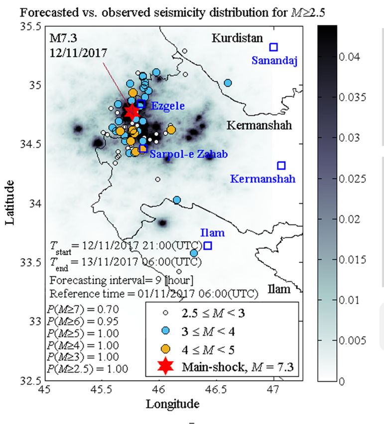
Starting Point                  Methodology             Application              Conclusion

Conceptual framework for quasi real-time hazard and impact forecasting within an ongoing seismic sequence in terms
 of occurrence, ground-shaking, damage, and losses in a prescribed forecasting interval (in the order of hours to days)

              Regional data, building inventory, population
             density, seismic micro-zonation, other required                    Quasi real-time earthquake catalog
              thematic maps related to the monitored area

             ETAS: Epidemic Type Aftershock                  Aftershock               Sequence-tuned updating of model
             Sequence model; spatio-temporal             occurrence model(s)                    parameters
          occurrence; every earthquake within the
         sequence is a potential triggering event for
         subsequent earthquakes by generating its                                          Operational forecasting of
           own Modified Omori aftershock decay.                                             aftershock occurrence

                                                           Ground motion               Forecasting of aftershock ground-
                                                         prediction model(s)                       shaking

                  This study                             Empirical/Analytical
                                                                                       Forecasting of aftershock damage
                                                          Fragility model(s)

                Retrospective early                        Loss model(s)                      Impact Forecasting
             forecasting of seismicity
            associated with the 2017-
             2018 seismic sequence                                                        Expected            Expected
             activities in western Iran                                                Financial Losses       Fatalities

     EGU21-15824
Starting Point         Methodology             Application            Conclusion

Fully simulation‐based framework for robust estimation of seismicity distribution
       in a prescribed forecasting time within an ongoing seismic sequence

 A Bayesian updating approach           A stochastic procedure is used in       The procedure leads to the
 based on an adaptive MCMC              order to generate plausible             stochastic spatial distribution of
 simulation technique is used to        sequences of events that are            the forecasted events and
 learn the ETAS model parameters        going to occur during the               consequently to the uncertainty
 conditioned on the events that         forecasting interval (the real          in the estimated number of
 have already taken place in the        sequence is unknown at the time         events, corresponding to a
 ongoing seismic sequence before        of forecasting).                        given    forecasting      interval
 the forecasting interval.                                                      (Robust seismicity forecasting)

           STAGE 01                                 STAGE 02                                STAGE 03
    Learning ETAS model parameters           Generating plausible sequences     Estimating spatial distribution of events

Ebrahimian H, Jalayer F (2017) Robust seismicity forecasting based on Bayesian parameter estimation for epidemiological
spatio-temporal aftershock clustering models. Sci Rep 7, 9803. https://doi.org/10.1038/s41598-017-09962-z.
Ebrahimian H, Jalayer F, Maleki Asayesh B, Zafarani H (2021) Operational aftershock forecasting for 2017-2018
Kermanshah seismic sequence in Western Iran. Bull. Seismol Soc Am (in Preparation).

     EGU21-15824
Starting Point Methodology Application Conclusion
The conditional rate of occurrence of events (the seismicity rate)
based on ETAS model
Kt Kr
ETAS t , x, y, m θ, seqt , Ml e mM K e
m M
l
j l
t t c r d
p q
2 2
t j t
j j
ETAS t , x , y θ,seqt ,Ml
The rate ETAS is at time t (with respect to a reference time), in the cell unit centered at the
Cartesian coordinate (x, y)A (where A is the aftershock zone), with the magnitude M≥m,
conditioned on:
the vector of ETAS model parameters [, K, , c, p, d, q].
the observation history up to the time t denoted as seqt={(tj, xj , yj, mj), tj
Starting Point Methodology Application Conclusion
Robust seismicity forecasting
E N x , y , m seq , M l N b x , y , m M l
Tend
T ETAS t , x, y , m θ, seq, M l dt p θ | seq , M l dθ
θ start
A robust estimate of the average number of events (E[·])
in the spatial cell unit centered at (x, y) with M≥m in the The conditional probability
forecasting interval [Tstart, Tend], which is calculated over density function (PDF) for
the domain of the model parameters . given the seq and Ml.
Nb(x, y, m|Ml): average number of events occurred due to the background seismicity with
magnitude M ≥m in the forecasting interval [Tstart, Tend].
IAT1 IAT2 IAT3 IATi Forecasting interval
Mainshock
To t1 t2 t3 ti Tstart Tend Time (t)
Sequence of events (seq) To ≤ ti
Starting Point Methodology Application Conclusion
Robust seismicity forecasting
E N x, y, m seq, Ml Nb x, y, m Ml
Tend
T ETAS t, x, y, m seqg, θ, seq, Ml dt p seqg | θ,seq, Ml dseqg p θ | seq, Ml dθ
θ seqg start
The robust estimate for the average number of aftershock events should also consider all
the plausible sequences of events seqg (i.e., the domain seqg) that can happen during
the forecasting time interval.
A plausible seqg is defined as the events within the forecasting interval defined as
seqg={(IATi =ti-ti-1, xi, yi, mi), Tstart≤ ti ≤Tend, mi ≥Ml}.
The use of the term “robust” here implies that a set of possible model parameters is used
to estimate the conditional number of events N(x, y, m|seq, Ml) rather than a single
nominal model parameter.
EGU21-15824Starting Point Methodology Application Conclusion
Robust seismicity forecasting
E N x, y, m seq, Ml Nb x, y, m Ml
Tend
T ETAS t, x, y, m seqg, θ, seq, Ml dt p seqg | θ,seq, Ml dseqg p θ | seq, Ml dθ
θ seqg start
This Equation can be solved via a fully simulation‐based framework:
• Vector of model parameters are sampled from p(|seq, Ml) using an adaptive Markov
Chain Monte Carlo (MCMC) simulation technique.
(1) The samples are used to generate plausible sequences seqg taking place within the
forecasting interval [Tstart, Tend] according to p(seqg| seq, Ml).
Note: The sequence of events that precede Tend is {seq, seqg}, where seq remains unchanged
(observed data) among plausible samples; Thus, a robust estimate for the average number of
events can be obtained based on the plausible model parameters.
EGU21-15824Starting Point Methodology Application Conclusion
About the model parameter K
m j Ml Kt Kr
ETAS t, x, y, m θ, seqt , Ml e m M l
K e
t t c r d
p q
2 2
t j t
j j
[, K, , c, p, d, q] ETAS t , x , y θ,seqt ,Ml
Method (a) Calculate K: Considering that K is directly affected by No (i.e., the number of events
taken place before the forecasting interval [Tstart, Tend]), it has an analytical closed‐form
expression, and its distribution can be derived based on other ETAS parameters. Thus, the vector
of model parameters has six parameters = [, , c, p, d, q].
Tstart IAT1 IAT2 IATi Forecasting interval
t, x, y θ, seq, M dx dy dt N
IAT3
Mainshock
l o
ti
To x, y A Total conditional intensity including To t1 t2 t3 Tstart Tend Time (t)
also background seismicity rate Sequence of events (seq) To ≤ tiStarting Point Methodology Application Conclusion
Kermanshah 2017‐2018 Seismic Sequence
Seismic Sequence from 11/01/2017 up to 01/12/2019
36
Kurdistan
35.5
M7.3 Sanandaj
35 12/11/2017 Ezgele M5.9
25/8/2018
34.5 Kermanshah
Sarpol-e Zahab
Kermanshah
Latitude
M6.3
34
25/11/2018
33.5 Ilam
Map of active faults of Iran (prepared by: B.
Maleki Asayesh, IIEES, Iran) 2.5 M < 3 Ilam
33 3MStarting Point Methodology Application Conclusion
Kermanshah 2017‐2018 Seismic Sequence
Ezgeleh MS Tazehabad event
Mw7.3 Mw5.9
12/11/2017 25/08/2018
To=01/11/2017
06:00 UTC
Sarpol‐e Zahab event
630 casualties, immense
Mw6.3
buildings’ damages and 25/11/2018
economic losses
From 12/11/2017 up to 18/04/2020 (i.e., in the time interval of around 2.5 years after the
Ezgeleh MS), about 9000 seismic events were recorded by Iranian Seismological Center, IRSC,
in the area shown in Figure. From this pool of seismicity, 2318 events have Mw≥2.5. In addition
to the Ezgeleh MS, 19 events with Mw≥5.0, and more than 125 events with magnitude larger
than 4 and less than 5 (4≤MwStarting Point Methodology Application Conclusion
Kermanshah 2017‐2018 Seismic Sequence
Ezgeleh MS Tazehabad event Sarpol‐e Zahab event
Mw7.3 Mw5.9 Mw6.3
12/11/2017 25/08/2018 25/11/2018
To=01/11/2017
06:00 UTC
Daily observed number of events (starting from 6:00 UTC each day)
100
M7.3 at 12/11/2017 - 18:18:16UTC
M5.0 at 20/11/2017 - 15:23:39UTC
80
Number of events
M5.5 at 11/12/2017 - 14:09:57UTC
60 M 2.5
40 M 3.0
20
0 7
7
7
7
7
7
7
7
7
7
7
7
-1
-1
-1
-1
-1
-1
-1
-1
-1
-1
-1
-1
ec
ec
ec
ec
ec
ec
ov
ov
ov
ov
ov
ov
-D
-D
-D
-D
-D
-D
-N
-N
-N
-N
-N
-N
02
07
12
17
22
27
02
07
12
17
22
27
EGU21-15824Starting Point Methodology Application Conclusion
Distribution of the ETAS model parameters (marginal PDF’s of posterior and prior)
with their statistics (mean and COV) after Mw 7.3 at 12‐November 2017
[Tstart, Tend]
(dd/mm‐hour)
c [day] p d [km] q K
sample mean=0.39 mean=0.04 mean=1.12 mean=1.36 mean=1.04 mean=208.40
[12/11‐21:00, prior COV=0.43 COV=0.29 COV=0.09 COV=0.19 COV=0.03 COV=0.34
13/11‐06:00]; ML=1.12
mean=0.99
Ml =2.5 COV=0.16
1 2 3 4 1 2 3 4 0.05 0.1 0.15 1 2 3 1 2 3 4 1 2 3 500 1000 1500
sample mean=0.64 mean=0.04 mean=1.11 mean=1.40 mean=1.05 mean=73.31
[13/11‐00:00, prior COV=0.24 COV=0.27 COV=0.08 COV=0.17 COV=0.03 COV=0.41
13/11‐06:00]; ML=1.21
mean=1.12
Ml =2.5
COV=0.12
1 2 3 4 1 2 3 4 0.05 0.1 0.15 1 2 3 1 2 3 4 1 2 3 200 400 600
sample mean=0.72 mean=0.04 mean=1.20 mean=1.46 mean=1.05 mean=31.41
[13/11‐06:00, prior COV=0.20 COV=0.30 COV=0.12 COV=0.18 COV=0.03 COV=0.33
ML=1.54
14/11‐06:00];
mean=1.50
Ml =3.0 COV=0.12
1 2 3 4 1 2 3 4 0.05 0.1 0.15 1 2 3 1 2 3 4 1 2 3 50 100 150
mean=MLE mean=2.00 mean=0.03 mean=1.10 mean=1.00 mean=1.50
Prior –
COV=0.30 COV=0.30 COV=0.50 COV=0.30 COV=0.30 COV=0.30
Note: To provide the forecast for each time window, the observation history, seq, comprises all the
events form To up to Tstart with M≥Ml. For the first forecasting interval (Tstart=12/11/2017‐21:00, i.e., 2
hours and 42 minutes after the main event) , the seq includes exactly 28 events with M≥2.5.
EGU21-15824Starting Point Methodology Application Conclusion
Seismicity forecasting
The forecasted seismicity maps (98%
confidence interval) for the number of events
with M≥Ml; the earthquakes within the
corresponding forecasting interval are
illustrated as coloured dots (distinguished by
their magnitudes) + main event of Mw7.3.
103 The observed (green star) vs. forecasted
92 number of events (error‐bar format) with
79
71 64 M≥Ml: the median value (the 50th percentile)
50 marked with a gray‐filled square; the 16th and
84th percentiles (marked with blue numbers);
the 2nd and 98th percentiles (marked with red
numbers).
P M m 1 exp E N x, y, m seq, M l dx dy
x , yA
The first seismicity forecasting map shows 9 hours
forecasting starting 2 hours and 42 minutes after
the main event.
EGU21-15824Starting Point Methodology Application Conclusion
Seismicity forecasting
61 73
55 61
49 53 50
43 41
34 39
32
The second seismicity forecasting map shows 6 The third seismicity forecasting map shows 24
hours forecasting starting 5 hours and 42 minutes hours forecasting starting around 12 hours after
after the main event. the main event.
EGU21-15824Starting Point Methodology Application Conclusion
Simplifications within the robust seismicity forecasting framework
ETAS model parameter K is estimated by a closed‐form expression in
method a, where the restricted condition that No events took place in
the aftershock zone at the time of starting the forecast is satisfied for
individual generated samples
Ir is solved Proposed
Calculate K (method a)
numerically Method
Integral over the whole
Semi-Fast
aftershock zone A: Calculate K (method a)
dx dy Method
r Approximated with I that
x , yA r d
2 2 q
is over infinite space; thus,
I 1
Learn K through the Fast
Bayesian Updating Method
(method b)
Relaxing the calculation of the spatial contribution of ETAS model
over the whole aftershock zone I (i.e., assuming I 1),
which manifests itself both in the likelihood estimation for
drawing the samples as well as generating the sequence seqg.
EGU21-15824Starting Point Methodology Application Conclusion Simplifications within the robust seismicity forecasting framework EGU21-15824
Starting Point     Methodology         Application       Conclusion

  Discussion on the effect of considering the integration over the
                      whole aftershock zone
(1) The first forecast, which might be the most important one (while less observed data is
    available at the time of forecasting), has higher dispersion and lower median by relaxing
    the estimation of I . This increase can mainly be attributed to the increase to some extent
    in the rate of rejection of samples through MCMC procedure. This is a key issue as there
    might be particular cases (not observed here in this case study), where this approximation
    results in biased estimates.

(2) As the sequence evolves, the difference between to two methods becomes negligible. This
    observation has been also made in Schoenberg (2013), where the assumption of an
    infinite spatial domain was shown to have negligible effect on likelihood.

(3) As a general observation within the five forecasting intervals in Table 3, the time of
    conducting the Semi‐Fast method is around 75% of the required time for performing
    Proposed method. Thus, Semi‐Fast method can be used to reduce the computational cost
    of calculating I , knowing that it may not be reliable for early forecasts after the
    occurrence of a main event.

   EGU21-15824
Starting Point Methodology Application Conclusion
Discussion on the effect of calculating K
(1) For the first and foremost forecasting interval, Fast method did not properly manage to
capture the number of events. This is mainly due to the lack of observed data used for
learning parameter K through MCMC procedure within the Fast method (note that ETAS
model parameters has 7 variables in this method). Thus, K becomes quite sensitive to the
choice of the prior (i.e., non‐informative prior does not work properly and the informative
prior forces the posterior distribution of K to follow similar trend to prior). This is by no
means a trivial problem and may cause significant underestimation in the early forecasts (as
can be seen in the first column of Fast method in Table 3).
(2) As the sequence evolves, the forecasts issued by the Fast method become more similar to
those obtained by Semi‐Fast method (and consequently the Proposed method). This is an
interesting observation showing that Fast method is reliable as the sequence evolves.
(3) Similar to Semi‐Fast method, this method is also exposed to high rate of sample rejections
through MCMC procedure which may lead to biased estimates.
(4) The time of conducting the Fast method is less than 50% of the required time for
performing Semi‐Fast method, making the procedure appealing (not reliable for early
forecasts after the occurrence of a main event).
EGU21-15824Starting Point Methodology Application Conclusion
Final Remarks
It is recommended to do the Proposed method at least for early forecasts. As the sequence
evolves, it is possible to do the Fast (or even the Semi‐Fast) methods. We observe that after
an initial transition time (in the order of few hours to accumulate enough events for updating
the model parameters), the model quickly and automatically tunes into the sequence and
provides forecasts that are reliable in most cases (the observed number of events are within
plus/minus one standard deviation of the distribution provided by the robust framework).
The Proposed method is quite efficient, and the most challenging first forecast (2 hours and
42 minutes after the main event) is performed around 40 minutes on a normal PC. Moreover,
the model updating and forecasting procedure is carried on without human interference and
use of expert judgement.
We have proposed a fully simulation‐based procedure for both Bayesian updating of ETAS
model parameters and robust operational forecasting of the number of events of interest
expected to happen in each forecasting time frame.
The robust seismicity forecasting framework herein is conditioned on the available catalogue
of events and the epidemiological model adopted for capturing the spatio‐temporal
aftershock clustering.
EGU21-15824Thank you for your attention! vEGU21: Gather Online | 19 – 30 April 2021
You can also read