Optimization of Rider Scheduling for a Food Delivery Service in O2O Business

Hindawi
Journal of Advanced Transportation
Volume 2021, Article ID 5515909, 15 pages
https://doi.org/10.1155/2021/5515909

Research Article
Optimization of Rider Scheduling for a Food Delivery Service in
O2O Business

 Guiqin Xue,1 Zheng Wang ,1 and Guan Wang1,2
 1
 School of Maritime Economics and Management, Dalian Maritime University, Dalian, China
 2
 Technical Unversity Bergakademie Freiberg, Akademiestraße, Freiberg 6,09599, Saxony, Germany

 Correspondence should be addressed to Zheng Wang; drwz@dlut.edu.cn

 Received 25 February 2021; Revised 6 April 2021; Accepted 1 May 2021; Published 25 May 2021

 Academic Editor: David Rey

 Copyright © 2021 Guiqin Xue et al. This is an open access article distributed under the Creative Commons Attribution License,
 which permits unrestricted use, distribution, and reproduction in any medium, provided the original work is properly cited.
 Services such as Meituan and Uber Eats have revolutionized the way the customer can find and order from restaurants. Numerous
 independent restaurants are competing for orders placed by customers via online food ordering platforms. Ordering takeout food
 on smartphone apps has become more and more prevalent in recent years. There are some operational challenges that takeout
 food service providers have to deal with, e.g., customer demand fluctuates over time and region. In this sense, the service providers
 sometimes ignore the fact that some riders may be idle in several periods in regions, while, in contrast, there may be a shortage of
 riders in other situations. In order to address this problem, we introduce a two-stage model to optimize scheduling of riders for
 instant food deliveries. A service provider platform expectantly schedules the least quantity of riders to deliver within expected
 arrival time to satisfy customer demand in different regions and time periods. We introduce a two-stage model that adopts the
 method of mixed-integer programming (MIP), characterize relevant aspects of the scenario, and propose an optimization al-
 gorithm for scheduling riders. We also divide the delivery service region and time into smaller parts in terms of granularity. The
 large neighborhood search algorithm is validated through numerical experiments and is shown to meet the design objectives.
 Furthermore, this study reveals that the optimization of rider resource is beneficial to reduce overall cost of the delivery. Takeout
 food service platforms decide scheduling shifts (start time and duration) of the riders to achieve a service level target at minimum
 cost. Additional sensitivity analyses, such as the tightness of the order time windows associated with the orders and riders’
 familiarity with delivery regions, are also discussed

1. Introduction are then prepared and packaged by restaurants, and the
 takeout delivery platform assigns independent contracting
Ordering takeout food on smartphone apps is becoming riders to deliver the food. Compared with other foodservice
more and more popular in China in the past several years. In providers such as McDonald’s and KFC, online food or-
a recent survey, 68% of diners order takeout food at least dering platforms do not hire a full-time employee to do the
once a day, with 33% order at least once a week [1]. The delivery job. Thus, a key issue faced by all takeout delivery
takeout delivery business is regarded as an online-to-offline platforms is how to formulate a timetable and route for
(O2O) business model applied by the food industry. In the riders to deliver food so that customers can get food as
past few years, Chinese consumers have widely accepted this quickly as possible within the desired time [2]. Besides,
model. Consumers could get rid of the hassle of going to taking into account the fluctuations in customer demand
restaurants but can get more food choices and faster services with regions and time periods, the scheduling of takeaway
through online ordering mode. In China, online takeout platforms will become more complicated. For example, the
food service platforms such as Meituan and Baidu provide order arrival rate usually fluctuates more during the peak
takeout ordering services to most of the working population. dining period (soaring during the meal times and dropping
Firstly, customers make orders on smartphone apps, meals to deficient levels in other mealtimes) in the business district

2 Journal of Advanced Transportation

than in the suburbs [3, 4]. Furthermore, to prevent or
mitigate any adverse effects of the uncertainty associated
with riders’ delivery capacity, the service platform may also
choose to have a scheduled delivery workforce that they can
utilize more effectively.
 Takeout service providers always try their best to fulfill
customer requirements in the delivery process. Customers
usually expect reliable and fast service within the expected
time [5]. Therefore, in this study, we developed and
evaluated a new approach to address order assignment and
riders’ service sequence. For the sake of simplicity, the rider
starts from the central depot to the restaurant in the rel-
evant pickup region. Generally, riders provide delivery
service for customers within a radius of 3 km. Customers 100
always place orders before each deadline, such as dividing
the day into equidistant service periods, 10 : 00–12 : 00, 12 : 0
 00–14 : 00, 15 : 00–17 : 00, and 17 : 00–19 : 00. We assume
that a restaurant receives an order at 10 : 30 with the Figure 1: The fluctuation of customer requirements over time and
deadline as 11 : 30. In this case, the service provider ob- space.
serves that the service region does not have adequate rider
resources, so the order is not assigned to the available rider time and space. However, in the nonmeal periods of a day,
to serve as fast as possible. The number of riders required some riders do not receive orders from the service provider.
varies in different periods in each region, and different There is excess capacity in this case. The expected delivery
regions have different order requests in the same period. time of orders is concise to a certain extent (the expected
Therefore, the delay of customer requests seems inevitable time refers to the customer placing the order to delivering
with the deadline. Furthermore, the delayed service also the order). Customers have more stringent requirements
leads to lower service quality and more customer com- than before the previous delivery system on speed, safety,
plaints [6]. Hence, a service platform needs to design and service quality. Therefore, the freshness of meals in the
reasonable scheduling plan to allocate riders’ resources for instant logistics delivery is becoming more significant than
instant food deliveries with respect to the fluctuations of the traditional transportation [6].
customer demand over time and space. As shown in Fig- Different types of ordering takeout have requirements
ure 1, colors from light to dark indicate customers’ ordering for distribution conditions and ways. Hence, they also
demand at the same ordering time. Meanwhile, it can be increase the difficulty of distribution processes for riders.
seen that the greater the customers demand near the central Besides, riders will flexibly adjust their routes according to
region, the smaller the demand in the edge region. their own experience and real-time road conditions. In
 Due to the practical challenges, instant logistics is facing doing this, the rider route usually deviates from the actual
many difficulties, while developing rapidly. Foodservice routes, and thus, this phenomenon delays the customer’s
providers face the complex problem as to control the cost of delivery service. A two-stage programming model is for-
scheduling riders, while maintaining high quality of cus- mulated to address the challenges mentioned above. In the
tomers’ service. That is, takeout service providers struggle first stage of the model, the rider’s fixed cost and the rider’s
to efficiently assign orders to riders for instant food de- travel cost are considered, and the second stage of the
liveries. The issue is an inherent contradiction between the model is to dispatch the rider to work in a specific area
undulated distribution of order time, space locations, and during a certain period. The study intends to provide a
available riders’ stability. Several regions will have excess reasonable solution heuristic to optimize the rider re-
idle riders/riders without delivery tasks during the trough, sources of service providers. We use the time series analysis
resulting in a waste of resources. However, during peak method to generate the initial route scheme according to
dining periods, the order volume shows an increasing trend the order quantity transmitted to the service provider. The
relative to nondining periods, and existing riders cannot consideration of the available riders in different periods and
satisfy the delivery demands of customers. This phenom- regions highlights the importance of punctuality [7].
enon is called insufficient rider resources. For example, in a Therefore, the objective of the first-stage is to minimize the
day, the two peak periods of ordering takeout are usually total cost, including fixed cost and traveling cost of riders in
12 : 00 to 13 : 00 and the dinner is 17 : 00 to 19 : 00, re- the subregion periods. The objective of the second-stage is
spectively. Moreover, the number of existing riders to minimize the rider scheduling times. The ordering
assigned by the service platform in regions is insufficient to takeout usually combines customer requests into a big
meet the growing customer requests. In this case, this order pool associated with the ordering time, space loca-
phenomenon always causes many orders which are not tion, food category, and freshness to deal with the order
delivered by the available rider resources for instant de- requests. Specifically, a service provider adopts a way to
liveries with fluctuation of customer requirements over assign orders and then schedules riders to deliver the

Journal of Advanced Transportation 3

distribution tasks in each period and subregion. This way algorithm is unreasonable to address the proposed problem,
usually refers to distribution regions. because the high timeliness of instant delivery. Therefore, in the
 The rest of the paper is organized as follows. In Section 2, real-world scenario, the heuristics approach is adopted. Ghiani
we review the related literature. We present the problem [26] introduced the order assignment and vehicle scheduling in
formally in Section 3 and formulate a multi-objective integer the dynamic dial-a-ride problem. Li (2016) proposed a large
programming model and its related definitions in Section 3. neighborhood search algorithm to address the share-a-ride
Section 4 details the solution to the proposed problem. We problem and determined the time slack. Klapp [27] formulated
use the proposed algorithm to perform the case study, of an arc-based integer programming model, and they also
which the data comes from a takeout platform in China. designed local search heuristics to solve a dynamic dispatch
Section 6 details the conclusion of this study and prospects waves problem where the order arrival times are known.
for future research opportunities. Gschwind [28] and Azi [29] developed a large neighborhood
 search heuristic to optimize the pickup and delivery problem.
2. Literature Review Gu [30] presented the benefits of the truck-drone combi-
 nation associated with the ordering takeout delivery of two
The delivery service providers deliver goods to customers over a advanced ant colony heuristics and a method to minimize the
given planning period [8]. They estimate the importance of number of dispatched vehicles and the total travel time. Besides,
transport capacity in the service regions to assign riders to deliver the same-day delivery is another subtopic of research worthy of
orders by the deadlines [5, 9]. To gain a competitive advantage, attention. When it comes to instant delivery, goods are usually
the instant delivery company tries the best to offer increasingly delivered within the same-day [6, 31]. These delivery activities
narrower delivery deadlines [10]. However, the trend towards always occur in the form of online behavior [32]. It is worth
shorter delivery lead-times increases transport resources cost for noting that the pickup node and delivery node are usually
the instant food delivery of customer requirements over period located in the same city. Ulmer [33, 34] analyzed the drones
and space, since the service provider has to recruit more riders combined with regular delivery vehicles to improve same-day
[11] or seeks the assistance of the third logistics, such as delivery performance based on geographical districting. Klapp
crowdsourcing [12–16] or spare social transport capacity [2], to [35] discussed the request acceptance and distribution decisions
release the transport resources pressure. Hence, transport ca- in same-day delivery. They split the time horizon into four-
pacity management is significant for the instant delivery pro- periods. Bent [36] applied the multiple-scenario approach
viders. [17–19]. Besides, Zhang et al. [20] analyzed the influence (MSA) to sample a set of scenarios for obtaining future cus-
of the pickers’ learning effects in the online integrated order tomer requests, and the samples can determine a suitable route.
picking and delivery application. They also consider the pickers’ Furthermore, in Table 1, we compare existing research works
learning effect essential for the order fulfillment process’s ac- with this study to show the main differences.
curacy and predictability. However, the riders will be passive The differences between this study and previous research
entities that are subject to a digital “panopticon” [7], as the effect are as follows. Firstly, we formulate a two-stage model to
is used to tame algorithms. Decisioners providing services need address the problem of configuring transport resources of
to maintain a balance by optimizing existing capacity resources, delivery riders and optimize both quantity and travel routes
that is, the balance between existing rider resources and service of the riders for fluctuations of customer demand over time
quality. In the case of rider resources and no additional riders are and space in any period of the entire region. Secondly, we
rented, the order requests of customers are delivered by design an LNS approach to generate the delivery rider’s
scheduling riders from other regions, while also ensuring the route given the determined minimum number of delivery
quality of customer service. riders in the first stage of our model. Then, the second stage
 The problem of instant delivery is closely related to the of our model is addressed by the Gurobi 9.1, a commercial
pickup and delivery problem [21] and the dial-a-ride problem solver. Thirdly, the service region and the whole day are
[22]. Each order has a pickup node and delivery node, re- divided into some subregions and subperiods.
spectively. Hence, the customer requires to be serviced by the Our contributions are as follows. Firstly, we present the
rider within an hour or less. For example, all riders must deliver optimization of rider scheduling for a food delivery service
the orders to customers within 45 minutes to take out the (ORSFDS) problem based on a dataset from an online-to-
delivery. Moreover, the rider must start from the depot, visit offline takeout food service provider in China. Then, we
some new pickup nodes that come up as a result of new formulate two MIP models and propose the LNS algorithm
delivery nodes, and then return to the depot within the given to generate the near-optimal solution. After that, an em-
time windows [23]. Otherwise, they may be subject to addi- pirical study and extended computation are carried out on
tional penalties due to delivery delays [24]. Usually, by using data provided by Dalian, China. Finally, this study includes
precise algorithms, we may work out the optimal solution, and the sensitivity analysis on the tightness of order time win-
by using the heuristic method, we may get a near-optimal dows and the rider’s familiarity with the region.
solution to the delivery problem. [25] discussed the rider
consistency in the dial-a-ride problem and proposed a branch- 3. Problem Definition and Formulation
and-cut algorithm to solve two mathematical formulations. To
the best of our knowledge, by exact methods, we may obtain the In this section, we first present a formal description of the
optimal solution. However, the computational time is too long ORSFDS. We then define the rider routing and rider scheduling.
for solving middle-size problems. Therefore, the exact Suppose a set of customers D � {1, . . . , d} that need to be

4 Journal of Advanced Transportation

 Table 1: Comparison between the existing literature and this study.
Reference Transport capacity Rider assignment Rider scheduling Two-stage model Heuristic algorithm
Ulmer et al. [33] √ √
So et al. [11] √ √
Berbeglia [21] √ √ √
Cordeau et al. [22] √ √
Li et al. [37] √ √
Archetti [8] √ √ √
Huang et al. [5] √ √ √
Steever et al. [38] √ √
Sun [7] √ √ √
Wang [39] √ √ √
Yildiz et al. [4] √ √
Liao [9] √ √ √
This study √ √ √ √ √

serviced by riders during time periods in regions, and they are Throughout this study, two decisions are to be made in
located in a connected graph, G � (V, E), where V � {0}⋃​ N this problem: the number of routes of riders and the service
is the set of vertices, E is the set of edges and N � P⋃​ D � periods and subregions of riders in the first stage of the
{1, . . . , n} is a group of nodes including restaurants and cus- model. For the number of riders and the traveling routes of
tomers. The node 0 represents the rider’s origin, and nodes 1 to n riders’ decisions, we use xr0j � 1 to indicate that riders
represent, respectively, the locations of restaurants and cus- deliver directly from 0 to j, that is, riders start from the
tomers. For each order i � (oi , di ), we use Os to denote the set of origin to work; and, xrij � 1 indicates that the rider travels
order sub-regions. In this study, we divide the distribution from i to j in the route, and xr0j � 0 and xrij � 0 ; otherwise,
region into several sub-regions and the rider service horizon into i, j � 0, 1, . . . , n. We also use xrst � 1 to denote that the rider
small time periods throughout the day. r provides delivery service for customer requests in the
 We present the fluctuation of customer demand with time period t in the subregion s during the working horizon. For
in a certain service region in Figure 2. The example is depicted in the sake of brevity, we formulate a two-stage model to
Figure 2. The figure shows the fluctuation of customer demand optimize the rider scheduling problem. The rider scheduling
with time in a specific service region. We discretize the working model is to determine the delivery route and number of
horizon of a day for riders and take every three hours as a period riders in each subregion during a time period and to de-
for riders to deliver meals. It can be seen from Figure 2 that there termine the working period and working region of a rider.
is excess capacity at T1 and T3 between the relationship of In practice, we consider several reasonable assumptions
rider’s supply and customer’s demand. Excess capacity refers to to guarantee model availability. (1) For each order, it has a
customers’ low demand at T1 and T3, resulting in some idle certain pickup quantity. Riders load the customer’s ordered
riders having no orders to deliver. However, at T2 and T4, there meals at the pickup node and unload them at the delivery
is insufficient capacity to meet customers’ demands. Insufficient node. (2) The pickup node is visited by the rider exactly once
transport capacity refers to the surge of customer demand in the later than the delivery node. Significantly, the pickup node
region at T2 and T4, and the existing riders cannot complete the and the delivery node must be accessed by the same rider. (3)
delivery of orders. Similarly, this phenomenon also exists in Each vehicle begins service at an initial position. As riders
other regions. Additionally, to make rational use of the existing are independent contractors, each rider determines how
resources, this study mainly considers integrating the existing assigned orders are sequenced and routed. (4) These routing
regional riders’ resources in a certain period to minimize the and sequencing procedures are known to the dispatchers.
scheduling cost and meet the needs of customers and service Since the order requests are known to the service providers
quality. Therefore, we develop a two-stage scheduling model to in advance, dispatchers and riders communicate via mobile
optimize the rider scheduling problem. phones. (5) Riders accept all orders assigned during the
 In practice, however, due to the sharp increase of order order horizon. The related notations and definitions used to
demand in the peak period (11 : 00–13 : 00 and 17 : 00–19 : formulate the ORSFDS are shown in Table 2.
 00), a service provider (e.g., Meituan) usually assigns
more riders to deliver orders within the expected time. To min : c1 xr0j + c2 dij xrij , (1)
assign resources more reasonably and thus attain low r∈Rs j∈N⋃​ {0} r∈RS i∈N j∈N
operation costs, we have developed a large neighborhood
search to solve the problem. In our study, in order to yroi � yrdi , ∀r ∈ Rs , i ∈ Os , (2)
alleviate the large amount of orders in the business dis-
trict, the existing rider resources cannot satisfy customers'
 yroi � 1, ∀i ∈ Os , (3)
order requests. Thus, we propose to schedule some idle r∈Rs
riders from a subregion with a small order volume to
another subregion with a large order volume to satisfy the
 tij + αir ≤ αjr + M 1 − xrij , ∀r ∈ Rs , i, j ∈ N⋃​ {0}, (4)
needs of customers in a timely manner.

Journal of Advanced Transportation 5

 Insufficient Insufficient
 Excess transport Excess transport
 capacity capacity capacity capacity
 T1 T2 T3 T4 Insufficient
 transport
 Excess capacity
 capacity

 Other areas
 Insufficient Excess
 Time transport capacity
 capacity
 0 3 6 9 12 15 18 21
 Supply
 Demand
 Figure 2: The fluctuation of customer demand with time in a certain service region.

 Table 2: Sets, parameters, and decision variables.
Notation Description
Sets
Rs Set of assigned riders in subregion
Os Set of orders in subregion, for any order i, it consists of two nodes, denoted by (oi , di ).
D Set of customers
S Set of sub-regions serviced by riders, S � 1, . . . , s
 Set of all nodes including pickup nodes (restaurant’s locations) and delivery nodes (customer’s locations) and the depot
N � P∪D∪O
 (the starting node of the rider)
Parameters
ai , bi The order placed time by customer i and the expected delivery time by customer i, respectively
uir The load quantity of rider r arriving at node i
αir Departure time of rider r at node i
qi The demand at node i
cr The capacity of the vehicle owned by the rider r
tij Each arc (i, j) is associated with a travel time
dij Distance of the arc (i, j), unit: meter
c1 Fixed costs for each rider, unit: CNY
c2 The traveling cost, unit: CNY
Decision
variables
xrij Binary decision variable equals 1 if the rider r travels from node i to node j; 0 otherwise.
 Binary decision variable equals 1 if rider r is assigned to deliver food delivery by the service platforms in the period t in
xrst
 the subregion s
yir Binary decision variable equal 1 if the rider r services node i

 ​
 αir ≤ bi , i ∈ D, (5) uir + qi ≤ ujr + M 1 − xrij , ∀i ∈ P, j ∈ N⋃{0}, r ∈ Rs ,

 αir ≥ ai , ∀i ∈ P, (6) (10)

 0 ≤ uir ≤ C, ∀i ∈ N, r ∈ Rs , (11)
αoi r + toi di ≤ αdi r, ∀i ∈ Os , r ∈ R, (7)
 xrij � yri , ∀r ∈ Rs , (12)
 xrdi oi � 0, ∀i ∈ Os , r ∈ Rs , (8) i∈N j∈N i∈N

 uir − qi ≤ ujr + M 1 − xrij , ∀i ∈ D, j ∈ N⋃​ {0}, r ∈ Rs , xrij � 1, ∀i ∈ N, � yri , ∀r ∈ Rs , (13)
 (9) r∈Rs j∈N i∈N

6 Journal of Advanced Transportation

 xrij � 1, ∀j ∈ N, riders at any subperiod in any subregion is denoted by qst .
 (14) There are |R| available riders in the distribution, denoted by
 r∈Rs i∈N
 R � {1, 2, . . . r}. We assume that each rider can only serve
 familiar subregions Sr ⊆S, Sr ≠ ϕ. Because of the fluctuations of
 xr0j � xr0j ≤ Rs , (15)
 r∈Rs j∈N r∈Rs j∈N
 order requests in different subregions and periods, riders who
 may transfer among subregions are denoted by s ∈ S to
 another s’ ∈ S. Each arc is associated with a transfer cost by
 xr0j � xrj0 ≤ 1, ∀r ∈ Rs , (16) css’ . Riders are not allowed to serve subregions far from their
 j∈N j∈N
 original region, and the rider has the maximum transfer
 distance Lmax . For the rider’s shift decision, the decision
 αir > 0, ∀i ∈ N, r ∈ Rs , (17) variable is denoted by xrst � 1, and the rider r provides
 delivery service for customer requests at a period t in the
 xrij ∈ {0, 1}, ∀r ∈ Rs , i, j ∈ N⋃​ {0}, i ≠ j, (18) subregion s. To satisfy the customer requirements and obtain
 the minimum scheduling times, the model is as follows.
 yri ∈ {0, 1}, ∀i ∈ N, r ∈ Rs , (19)
 min � xrst , (20)
 r∈R s∈S t∈T
 The objective function (1) seeks to minimize the total
costs, including fixed cost and riders’ travel cost [40]. Con-
straints (2) and (3) ensure that each order in the subregion is xrst ≤ 1, ∀r ∈ R, t ∈ T, (21)
 s∈S
serviced exactly once by the same rider from the pickup node
to the delivery node. Constraint (4) satisfies the travel time
requirement between two adjacent nodes. Constraint (5) xrst ≥ qst , ∀s ∈ S, t ∈ T, (22)
 r∈R
guarantees that customer requests are delivered before the
order expected delivery time. The rider arrives at the res-
 xrst � 0, ∀r ∈ R, t ∈ T, (23)
taurant to pickup food or leaves the restaurant to deliver food
 s∈S/Sr
after placing the order is presented in constraint (6). Con-
straint (7) presents the time relationship between the same
rider visiting the pickup node and delivery node; That is, the xrst + xrs′ (t+1) ≤ 2, ∀r ∈ R, s, s′ ∈ S, t ∈ T, css′ ≤ Lmax , (24)
delivery time when the rider leaves the delivery node cannot
be earlier than the total time. It is determined by the pickup xrst + xrs′ (t+1) ≤ 1, ∀r ∈ R, s, s′ ∈ S, t ∈ T, css′ > Lmax , (25)
time and traveling time from the pickup node to the delivery
node. The arc does not travel directly from the pickup to the xrst ∈ {0, 1}, ∀r ∈ R, s ∈ S, t ∈ T. (26)
delivery node, as in Constraint (8). Payload capacities are
presented in Constraints (9)-(11). Constraints (9) and (10) The objective function (20) minimizes the overall sched-
define the payload capacity of the vehicle owned by a rider. uling time of riders [16]. Constraints (21) ensure that each rider
Constraint (11) determines the payload does not exceed the can serve at most one subregion at a period. Constraints (22)
capacity of the vehicle. Constraint (12) shows the relationship indicate that the number of riders required by each sub-region
between the node and the rider’s ownership. Constraints (13) in each period is not greater than the total number of assigned
and (14) ensure the connectedness of the order nodes. riders. Constraints (23) state that each rider has a fixed familiar
Similarly, constraints (15) and (16) indicate that each rider region and cannot go to the unfamiliar sub-regions. Con-
starts from the depot, goes to the restaurant to pickup food, straints (24) and (25) govern the transfer distance relationship
delivers the customer request, and returns to the same depot. for riders. Finally, Constraints (26) denote the decision variable.
Constraints (17)-(19) are decision variable definitions.
 Riders’ shifts are crucial for the optimization of the 4. Solution Heuristic
scheduling of riders. However, in the real-world scenario,
the number of riders required is different in each period and This section introduces the proposed large neighborhood
each subregion. For example, at two peaks throughout the search algorithm in detail. There are some metaheuristic
day, the number of order requests increased almost expo- algorithms that may have several drawbacks such as pre-
nentially. In this case, the number of riders required for each mature convergence and to tramp in local optimal or
period in the same region varies over time. Therefore, we stagnation. To overcome these disadvantages, this study
propose a new way of scheduling riders. In other words, we attempts to develop a hybrid heuristic algorithm that enables
schedule idle riders from several subregions to other sub- it to acquire high computational efficiency. Furthermore,
regions with less transport capacity in the same period so heuristics and metaheuristics are widely applied for different
that the problem attaining the case of short riders in some research domains, such as online learning, scheduling,
subregions during the peak period could be solved. multiobjective optimization, medicine, passenger and
 For the sake of simplicity, in the second stage of the freight terminal operations, data classification, and others.
model, we suppose a set of subregions that need to be serviced As far as we know, the proposed rider scheduling model
by riders during the period. In our discussion, we assume a set is an extension of the dial-a-ride problem, a well-known NP-
of periods T � t1 , t2 , . . . , t|T| , and the payload capacity of hard problem [41]. Therefore, it is crucial to obtain high-

Journal of Advanced Transportation 7

quality optimization results in a reasonable calculation time. Table 3: The pseudo code of the heuristic algorithm.
A large neighborhood search algorithm is a widely verified Input: The order dataset
resource scheduling algorithm [42]. The constructed initial Output: The numbers of the riders and the rider’s route
solution improves the existing solution by iteratively exe- Step 1: generate initial route sini by using insertion heuristic
cuting the destroy and repair operators and generates an Step 2: set initial solution sini as the current solution,
approximately optimal solution. neighborhood solution snei , and best solution sbest
 In the rider scheduling model, we optimize both the Step 3: implement remove operation on current solution scur to
number of riders and the route of riders. Firstly, we design an obtain partial solution spart
insertion heuristic method to construct feasible initial solutions Step 4: use repair operator to obtain neighborhood solution snei
 from partial solution spart
quickly; in the subsequent iterations, the existing solutions are
 Step 5: if snei outperforms sbest , accept the inferior solution
destroyed by the removal operator, and then the removed according to the principle of simulated annealing
orders are inserted by the repair operator. After this operation, Step 6: check if the termination condition is fulfilled, that is, after
a new neighborhood solution can be generated from the N consecutive iterations, the value of S_best no longer changes.
current solution. When the termination condition is satisfied, Then, jump to step 6 if yes, otherwise to step 3
the algorithm outputs the optimal solution. Table 3 shows the Step 7: output the optimal solution
pseudo-code for designing a large neighborhood algorithm.
 implement repair operators to construct a new feasible solution
4.1. Insertion Heuristic to Design Initial Solution. Cordeau from partial solutions. In this study, useful repair operators are
et al. [41]constructed an initial solution using the com- the optimal insertion operator, regret insertion operator, and
pletely stochastic method. However, the downside of this maximum waiting time insertion operator.
method is sometimes the infeasible solution may also be
obtained. Therefore, in the proposed, we consider the time
 4.2.1. Remove Operator. The purpose of the neighborhood
window of orders and the proximity of orders to generate a
 search is to remove some orders from the current solution
rider’s feasible route quickly. First, all orders are sorted
 based on specific criteria. There are four neighborhood
ascendingly based on the expected arrival time of the or-
 operations applied in this study as follows.
ders; then, each order is assigned to the rider’s delivery
 Natural sequence removal operator: the node in the route
route to generate |R| initial sequences according to ex-
 with “0” rider load is referred to as the natural sequence. In
pected arrival time (from early to late). Finally, we merge
 general, the rider route consists of two natural sequences, re-
the orders into the same delivery route by taking care of the
 spectively. That is, sequence 1 ⟶ 2 ⟶ 1 + n ⟶ 3 ⟶ 2 +
four metrics listed below:
 n ⟶ 3 + n and sequence 4 ⟶ 5 ⟶ 5 + n ⟶ 4 + n, namely.
 (1) Calculate the distance between two pickup nodes. Randomly selects a natural sequence from the removal operator
 and removes it from the current rider route.
 (2) Calculate the distance between two delivery nodes.
 Maximum time window removal operator: select the
 (3) Calculate the distance between a delivery node and a order with the largest time window in all routes and remove
 pickup node. them because orders with larger time windows have more
 (4) Calculate the distance between a pickup node and a time flexibility.
 delivery node. Worst order removal operator: for the rider route, the
 removed route’s cost-saving value calculates one by one and
 Delivery route merging is performed iteratively. In each removes the order with the most considerable saving value.
iteration, an order is randomly selected from the remaining Cluster removal operator: randomly select a root node
uninsured orders, one of the four metrics is randomly selected, and threshold, and then remove the order on each route
the minimum distance based on these two random features is closest to the root node.
then calculated, and the order is inserted into the route with the
minimum distance. During the insertion process, we also need
to do a feasibility check according to the constraints of the 4.2.2. Repair Operator. The purpose of the repair operation
order assignment’s model to ensure the feasibility of the initial is to reinsert the removed orders into the rider route. The
solution. A feasible initial scheduling plan is obtained until all repair operator performs iteratively in the repair process
orders are inserted into the route. until all orders insert into a set of routes. In this study, we use
 the following three kinds of repair operators.
 Optimal insertion operator: this way is similar to the
4.2. Neighborhood Search. In this section, to obtain a new insertion heuristics operation in section 4.2, in which the
neighborhood solution, the removal operation and repair unserviceable orders insert to the location of the minimum
operation are designed by destroying and reconstructing the cost increment.
current solution. In the removal operation, we use four removal Regret insertion operator: considering the optimal cost
operators: natural sequence removal operator, maximum time value insertion, the most challenging order usually puts to
window removal operator, worst order removal operator, and the final processing. Therefore, for all unserviceable orders,
cluster removal operator. As with each removal operation, the the optimal insertion location’s cost value is calculated and
output result is only a part of the solution. Therefore, we generated by the cost value vector. Then, randomly select a

8 Journal of Advanced Transportation

value from the vector and insert its corresponding order into Table 4: Summary of results on different scale instances.
the route. TS LNS
 The optimal
 The maximum waiting time insertion operator is to Ins. qi Q
 solution Solution Time Solution Time
insert orders into the rider route with a more considerable
buffer time. The waiting time refers to the time difference a2-16 1 3 2 2 10 2 17
Δtwait � αir − ti , ∀i ∈ P, between the rider’s arrival time and a2-20 1 3 2 2 16 2 16
the pickup node’s opening time. a2-24 1 3 2 2 20 2 29
 a3-30 1 3 3 3 26 3 30
 a3-36 1 3 3 3 28 3 32
 a4-40 1 3 4 4 32 4 34
4.3. Selection and Stopping Criterion. The optimal and regret
 a4-48 1 3 4 5 35 5 43
insertion is used to generate the initial feasible solution b3-24 U[1, 6] 6 3 3 18 3 25
based on its current number. At each iteration of the al- b3-30 U[1, 6] 6 3 3 24 3 30
gorithm, we randomly select removal and repair operators to b3-36 U[1, 6] 6 3 3 27 3 29
destruct and reconstruct the current solution and obtain a b4-16 U[1, 6] 6 4 4 10 4 12
new solution. Moreover, the simulated annealing criterion is b4-32 U[1, 6] 6 4 4 26 4 30
used to determine if the new solution is accepted. Therefore, b4-48 U[1, 6] 6 4 4 35 4 41
by adopting this criterion, we can accept a suboptimal so- b5-40 U[1, 6] 6 5 6 32 5 32
lution for the time being to search for a universally optimal b5-50 U[1, 6] 6 5 6 38 5 40
solution rather than a locally optimal solution. b5-60 U[1, 6] 6 5 5 42 6 50
 b6-48 U[1, 6] 6 6 7 34 7 39
 b6-60 U[1, 6] 6 6 7 40 7 49
5. Computational Experiments and Analysis b6-72 U[1, 6] 6 6 8 44 7 45
 b7-56 U[1, 6] 6 7 8 41 7 44
5.1. Benchmark Example Test. The LNS algorithm is b7-70 U[1, 6] 6 7 9 46 8 46
implemented in C# and tested on a system with 64bit b7-84 U[1, 6] 6 7 9 55 8 60
Windows 10 OS, Intel i7 processor (2.60 Hz), and 16 GB b8-64 U[1, 6] 6 8 9 43 8 52
RAM. Then, we use the Gurobi 9.1.0 commercial solver to b8-80 U[1, 6] 6 8 9 53 9 68
verify our model, but it can only handle less than ten orders. b8-96 U[1, 6] 6 8 9 73 9 82
Therefore, we need to adopt the proposed heuristic to solve
medium-sized problems.
 The DARP has been studied for decades, associated with LNS algorithm is stochastic in nature, and their performance
many benchmark instances that have been given. The often fluctuates, so for test instance (a) and instance (b), we
standard instance provided by Cordeau [22] is used to verify run the proposed algorithm for 1000 iterations. The con-
the proposed mathematical model and heuristic method. vergence processes are shown in Figure 3; although the
 The difference between the proposed algorithm and convergence rate of the LNS algorithm is slow, the solution
DARP is that the pickup node and delivery node have only a approach has good stability. It should be noted that instance
one-sided time window. Therefore, the standard DARP (a) and instance (b) are the benchmark examples, whose
instance can quickly be transformed into a test instance convergence is shown in, namely, Figures 3(a) and 3(b). In
based on the first-stage of the model. We can set the time the real-world scenario, the time difference between the two
window on the right side of the pickup node and the delivery algorithms can be ignored. Therefore, the LNS algorithm in
node’s left side as positive infinity and 0, respectively. this study can better solve the first stage of the model.
 We have compare the tabu search with the proposed LNS
algorithm, and the results are shown in Table 4. The first 5.2. Data Source. This section is about ride optimization
column shows the instance name. The second column scheduling problems for on-demand food deliveries with a
enumerates the order requests. Inset A, the quantity of computational experiment from Dalian, China. Section 4.2.1
customer requests is one unit. However, set B is subject to analyzes the delivery company’s order data in half a month
the uniform distribution. The third column is the capacity of to illustrate customer demand fluctuations in time and
the rider’s vehicle. Column 4 indicates the minimal number space. In Section 4.2.2, this study carries out a specific
of riders obtained from the model. Columns 5 to 6 and 7 to 8 calculation test to optimize riders’ transport capacity. Sec-
denote the tabu search and LNS algorithm’s solution and tion 4.3 discusses sections of discusses window tightness and
computational time, respectively. riders’ familiarity with distribution regions based on ca-
 According to Table 4, the proposed algorithm and tabu pacity assignment.
search method are two implementations of the first stage of
the model. The performance of the proposed algorithm is
better than the tabu search algorithm. We could obtain an 5.2.1. Description Of Real-World Cases. In this section,
optimal solution for 16 of the 24 instances by using the LNS numerical experiments are performed based on data from an
algorithm; however, by employing the TS algorithm, we online-to-offline food delivery platform located in Dalian,
could only get an optimal solution of 13 instances. However, China. To demonstrate the proposed algorithm’s effective-
in terms of the computational time, the LNS algorithm is ness in the configuration of transportation resources of
slightly longer than the tabu search algorithm. Moreover, the delivery riders for on-demand food deliveries with the

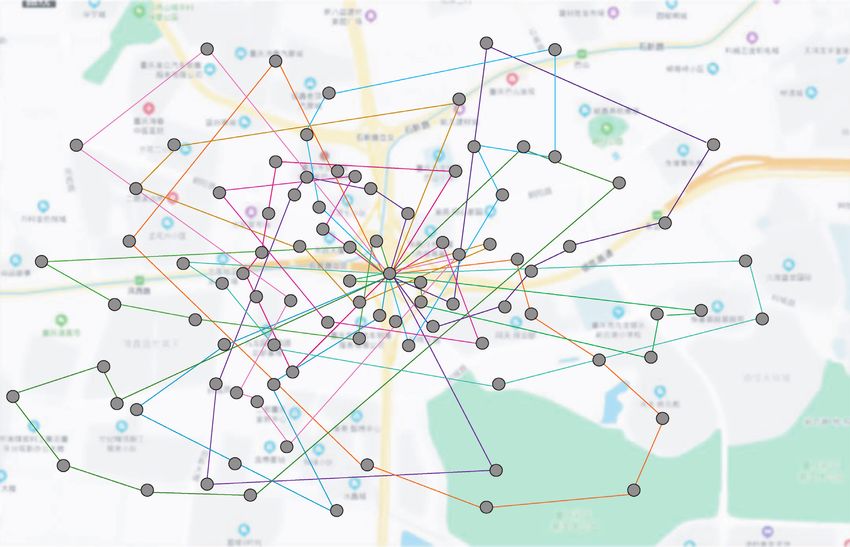
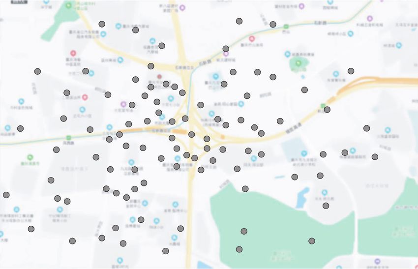
Journal of Advanced Transportation 9

 16

 15 18

 14
 16
 13
 Objective value

 Objective value
 12 14

 11
 12
 10

 9
 10
 8

 7 8
 0 200 400 600 800 1000 0 200 400 600 800 1000
 Iteration Iteration

 TS TS
 LNS LNS
 (a) (b)

 Figure 3: The convergence processes for instances. (a) Instance b8-64 (b) Instance b8-96.

fluctuations of customer demand over time and space, we required. The coordinates of the rider resource based on the
take the customer order requests of a takeout food service Baidu Map are shown in Figure 7. No. 0 stands for the
provider from January 1 to 15, 2017, as the data source. Data depot. The order pickup nodes are from No. 1 to No. 46,
sources include order IDs, restaurant names, customer lo- and the corresponding delivery nodes are from No. 47 to
cations, rider names, order times, delivery times, navigation No. 92. The demand for each order is 1 unit, and the ca-
distances, order regions, and rider regions. Then, we use the pacity of the rider is six units. The fixed cost of the rider is
Python pandas package to process the data and get all order 150 CNY.
requests from the first 15 days of Jan 2017, as shown in The proposed LNS algorithm is implemented in C# and
Figure 4. It can be observed that the average number of daily run on an environment with Intel(R) Core (TM) i7-9750H
orders is more than 5000. CPU, 2.60 GHz, and 16 GB of RAM. The minimum number
 Furthermore, the business districts with more than 100 of riders is 13 in the above instance. The routes of riders are
orders on January 1, 2017, are selected as our research re- shown in Table 5 and Figure 8. Therefore, the first stage of
gions. Then we get 23 sub-regions, and their detailed the proposed model and the LNS heuristic are effective for
information is shown in Figure 5. There are very few or- the takeout food service provider in reducing the number of
ders taken before 8 : 00 AM and 20 : 00. The peak hours are delivery drives required in the given period.
11 : 00–12 : 00, 14 : 00–15 : 00, and 16 : 00–17 : 00. As a result, Moreover, in Table 6, we present the minimal number of
we focus on the delivery period from 8 : 00–20 : 00. We riders obtained by the proposed heuristic and the number of
divide the whole day into six sub-periods, and each sub- dispatched riders in an original dataset in the 23 subregions
period is 2 hours. from 10 : 00 to 12 : 00. The results show that, in 20 out of 23
 To analyze the order requests imbalance among the subregions, our method outperforms the current system in
different sub-periods and sub-regions. We select four use. Therefore, we conclude that the proposed model and
business districts: Luosifu, Xi’an Road, Wanda, and LNS algorithm are superior to the current assignment
Shandong Road, to depict the order variations in Figure 6. method. Furthermore, we optimize the number of riders in
We could see that the number of orders made by cus- the six time periods and 23 subregions. We assume that the
tomers varies in regards to both time and region. transfer distance between two adjacent subregions is 3 km.
Therefore, the takeout food delivery platform needs The maximal allowed transfer distance for each rider is 9 km
reasonably schedule riders to deliver customer requests between two consecutive subperiods. The Gurobi 9.1 solver
and maintain the transportation capacity at a suitable is used to generate the optimal solution for the second stage
level. of the model. The corresponding results are presented in
 Table 6.
 Table 7 presents the minimal number of riders required
5.2.2. Optimization of Rider Scheduling. This section selects of the 23 subregions in the six subperiods. However, the
46 orders from 10 : 00 to 12 : 00 in the Luosifu business instant delivery network needs 300 riders, and all riders
district to determine the optimal number of delivery riders schedule 1800 times. However, in the real scenario, a

10 Journal of Advanced Transportation

 7500

 7000

 The number of the orders
 6500

 6000

 5500

 5000
 0 2 4 6 8 10 12 14 16
 Date
 The number of the orders
 Figure 4: The average daily orders in the first half of January 2017 based on the historical dataset.

 6000 1000

 The number of the orders in each hour
 5000
 800

 4000
 The cumulative orders

 600
 3000
 400
 2000

 200
 1000

 0 0

 4 6 8 10 12 14 16 18 20 22 24
 Time

 Cumulative demand
 Demand of each period

 Figure 5: The statistics chart of the orders in January 2017.

service provider assigns 328 riders and schedules 2180 time periods in the same region. For example, No. 1 assigns
times to deliver customer requests. In order to address the a rider to deliver orders in 6 different subregions. Hence,
fact that existing riders cannot satisfy the customer's or- configuring riders’ transport resources for instant deliv-
dering demands during the peak meal period, in our study, eries with the imbalance of customer requirements over
we proposed to schedule idle riders from some subregions time and space is extremely critical.
to other subregions with high rider’s demand. In this way,
the total number of riders has been reduced by 8% com-
pared to the previous scheduling scheme (each subregion 5.3. Sensitivity Analysis. In this section, we conduct sensi-
has sufficient riders), and the cost of scheduling riders has tivity analysis on the tightness of the order time windows
also been saved by 4200 CNY. Hence, good capacity op- and regional familiarity.
timization is practical and economical for service pro-
viders. Randomly select ten riders and discuss the rider’s
changes in the service area in subperiods, and the results 5.3.1. Analysis on the Tightness of the Order Time Windows.
are shown in Table 8. The results show that the number of Punctuality is crucial to on-demand food delivery businesses
riders required in different time periods in different sub- since the freshness of meals must be preserved within the
regions is different. This is due to the fluctuation of orders scheduled arrival time to meet the customers’ expectations.
in the same time period in different regions and different Besides, by introducing an optimal delivery riders schedule,

Journal of Advanced Transportation 11

 18 17
 16 16 15 15
 14

 The number of the riders
 14 14 13
 12 13
 12
 12
 10 10 10
 10 9 9
 8 8 9
 8
 6
 6 6

 4 4
 3
 2 2

 8:00~10:00

 10:00~12:00

 12:00~14:00

 14:00~16:00

 16:00~18:00

 18:00~20:00
 Subperiod

 Luosifu Xi’an road
 Wanda Shangdong road
 Figure 6: Statistical chart of transport capacity demand in each subperiod of the business circle.

 52 7 62

 8 44 37

 45
 64 39 90 41
 71 43 49
 2 29 42 67
 83 86 5
 35 36 89
 47 6 40
 17
 34
 75 15 66 81 61 63
 25 24 33
 70 78 4
 21 0 53
 73 68 60
 50
 28 18 85
 13 58 3 38
 56 46 65 12
 88 84 22
 59 23
 20 9 69 91 80
 11 1 14
 48 10 27 19
 87
 57 55
 79 6
 32
 92
 26 31
 82
 51 76 74
 54 77
 30
 72

 Figure 7: The spatial distribution of 46 orders.

more operation costs can be saved for the delivery platforms. the objective is to satisfy all customer requests to obtain a
However, in the most extreme cases, one order is assigned to good service reputation. We simulate three different order
one delivery rider only by the takeout service platform since time windows and discuss the number of riders required.

12 Journal of Advanced Transportation

 Table 5: Optimization of rider scheduling.
Rider index Rider routes
1 0-1-21-25-47-71-67-0
2 0-12-22-14-58-60-68-0
3 0-4-23-27-69-73-50-0;
4 0-41-5-30-76-51-87-11-57-0
5 0-24-70-13-59-20-66-0
6 0-16-45-44-62-43-90-89-91-0
7 0-37-39-83-15-85-61-0
8 0-33-46-92-6-79-18-64-52-0
9 0-29-8-75-31-54-77-32-19-65-78-0
10 0-40-86-2-36-28-48-74-82-0
11 0-34-42-35-88-80-81-0
12 0-3-7-49-17-63-53-38-84-0
13 0-9-55-26-72-10-56-0

 52 7 62
 8

 44 37

 64 39 45 90 41
 71 43 49
 29 67
 2 42 5
 35 86 89
 83 36 40
 47 6
 17
 34 66
 75 15 81 61 63
 70 25 33 78 4
 24 0
 50 68 60 53
 13 21 18
 73 28 58 3 38 12
 85 56 65
 88 84 23
 20 46 22
 9 69 80
 11 59 91 14
 48 10 1 27 19
 87 57
 79
 6
 55 32

 51 26 92 31
 82
 76 74
 54 77
 30
 72

 Figure 8: Visualization of the rider’s scheduling route.

Case 1 is the relaxed time windows, and the rider only has 60 number of riders are closely related. More importantly, tighter
minutes. Case 2 is the standard time window, and the rider time windows will inevitably make the distribution of transport
has to go from the pickup node to the delivery node in capacity more imbalanced because the food delivery platforms
45 minutes. Case 3 is the tight time windows, and only 30 have to assign more riders in peak periods.
minutes is allowed. We test the three different time windows
in the Luosifu business district, and the corresponding re-
sults are shown in Figure 9. 5.3.2. Analysis on the Regional Familiarity. In the second-
 As the time window tightens, Figure 8 displays an opposite stage of the model, we prohibit the riders from visiting the
trend between the number of dispatched riders and each rider’s sub-regions’ orders they are not familiar with regions. Be-
average order number. A more relaxed time window means cause riders may spend less time to finish orders in a more
fewer riders and more orders for each rider. Overall, the results familiar region, in the previous instance, we use the routes
show that the tightness of the order time windows and the provided by Baidu Map, but there may be other shorter

Journal of Advanced Transportation 13

Table 6: Number of riders in 23 sub-regions for instant deliveries. Table 8: Regional scheduling of some riders in each period.
 The number of the riders after The actual used The rider number
No. Sub region number
 optimization riders 1 2 3 4 5 6 7 8 9 10
1 18 19 1 0 0 0 0 0 0 0 1 1 1
2 16 17 2 3 1 0 2 0 1 0 0 0 0
3 17 18 3 6 4 1 1 2 4 2 0 0 0
4 14 15 4 9 1 2 3 3 6 4 1 0 0
5 13 16 5 11 1 2 1 1 4 6 4 0 0
6 14 15 6 13 4 2 3 4 4 8 2 0 1
7 17 19
8 14 17
9 14 14 18
10 17 18

 The average order numbers of each rider
11 14 16 4 17 4.0
12 15 15 16

 The number of the used riders
13 18 21
 3.5
14 13 14
15 14 15 14
16 14 17 3 3.0
17 16 16 13
18 13 15 12
19 15 16 2.5
20 12 14
 10
21 14 16
22 17 20 2 2.0
 9
23 14 16 8
 One Two Three
 Case

 The number of the used riders
 The average order numbers of each rider
Table 7: The minimum number of riders required for each sub-
region and each period of the whole delivery day. Figure 9: Relationship between the number of riders and the
 number of orders per capita under different time windows.
 Subperiod number
Sub region number
 1 2 3 4 5 6
1 7 13 7 9 12 7 55
2 14 6 7 8 7 13
3 13 15 13 9 7 13 50
4 12 5 7 12 8 8 45
 The required number of the riders

5 11 13 13 13 14 12
6 13 12 10 13 11 6 40
7 10 13 9 11 14 10 35
8 12 9 10 14 8 6
9 6 11 9 8 14 14 30
10 5 14 7 14 13 6 25
11 12 19 12 14 12 20
12 14 19 18 18 14 15 20
13 12 18 16 20 12 18 15
14 12 15 13 17 13 14
15 10 12 13 15 20 12 10
16 18 12 19 10 10 18 5
17 14 15 12 16 13 15
18 17 17 18 13 17 16 0
 0 1 2 3 4 5
19 18 12 19 15 20 17 Regional familiarity
20 15 10 10 15 14 20
21 5 8 7 9 13 6 The required number of the riders
22 7 15 12 14 15 10
 Figure 10: Relationship between regional familiarity and the re-
23 14 6 9 13 6 14
 quired number of riders.

14 Journal of Advanced Transportation

routes in practice. Therefore, we define the regional famil- considerations, may outperform the proposed way in this
iarity to describe the radio between the Baidu Map distance study model, in terms of optimizing service resources.
and the rider’s actual travel distance. It is evident that the There are several directions for further research. Firstly,
smaller the familiarity, the larger the actual travel distance. we will consider the order demand mode of different de-
We still take the Luosifu as an example and discuss the livery areas and the historical fluctuations of order demand
transportation capacity fluctuations in different regional in peak and off-peak periods, weekdays, and holidays.
familiarity. The results are depicted in Figure 10. Secondly, appropriate resource partition methods are
 In Figure 10, the delivery system’s number of delivery designed to optimize the allocation and scheduling of dis-
riders increases with the regional familiarity. When the rider tribution-driven subareas. At last, the uncertainty in the
maintains a higher regional familiarity, the required rider delivery process may be considered (such as the uncertainty
will be smaller, which will reduce the transportation capacity of order extraction (unexpected delay and real-time traffic
demand. Otherwise, the company assigns more riders, or the conditions) to propose a more robust solution. Overall,
rider must travel a longer distance, which will increase the considering more uncertainties, the on-demand food dis-
transportation capacity burden. tribution-driven scheduling problem may also be worth
 studying.
6. Conclusions
 Data Availability
This study introduced a two-stage model to tackle riders’
optimization problems in the on-demand food delivery The data used to support the findings of this study are
business. Considering the intensively fluctuating demand of available from the corresponding author upon request.
customer orders regarding period and region, the whole
municipal level region is divided into smaller sub-regions Conflicts of Interest
while the whole period is divided into several sub-time pe-
riods. For each subregion, we formulate a dial-a-delivery rider The authors declare that there are no conflicts of interest
model (first-stage of the model of our model) to minimize the regarding the publication of this paper.
delivery riders’ number in each period. Furthermore, the
imbalance of transportation capacity in different sub-regions Acknowledgments
and sub-periods is considered, and a transportation capacity
 This work was supported by the National Natural Science
allocation model (the second-stage of our model) is then built
 Foundation of China (71971036, 71421001, and 71531002),
to minimize the time of the delivery rider’s schedule. Due to
 the Major Program of Key Disciplines in Dalian
the computational complexity of the first-stage of the model,
 (2019J11CY002), the Key R&D Project of Liaoning Pro-
we develop an ALNS heuristic to generate a near-optimal
 vincial Department of Science and Technology (2020JH2/
solution. In the next step, we have compared our proposed
 10100042), and the Humanities and Social Sciences Program
heuristic with results from other studies. Finally, the second-
 of the Ministry of Education of China (19YJA630084).
stage of the model is solved by Gurobi 9.1, a commercial
solver. The dataset from an O2O foodservice platform in
China is used to conduct the case study.
 References
 The results show that fewer delivery riders are required [1] Iimedia, “Research report on china’s online catering takeout
than the current delivery system in use by applying the first- industry in the first half of 2017,” 2017, https://www.iimedia.
stage of the model. The cost of saving after applying our cn/c400/54716.html.
model is 4200 CNY, and the new plan of delivery rider [2] B. Kin, T. Ambra, S. Verlinde, and C. Macharis, “Tackling
scheduling reduces the total delivery times by 328. Hence, fragmented last mile deliveries to nanostores by utilizing spare
 transportation capacity-A simulation study,” Sustainability,
the proposed model and algorithm could optimize the
 vol. 10, no. 3, p. 653, 2018.
number of delivery riders in each subregion and improve the [3] Reuters, “How Amazon Is Making Package Delivery Even
delivery rider scheduling. Besides, we find that the tightness Cheaper,” 2016, https://fortune.com/2016/02/18/amazon-
of the order time windows and the number of delivery riders flex-deliveries.
are closely related, and a tighter time window means more [4] B. Yildiz and M. Savelsbergh, “Service and capacity planning
delivery riders and fewer orders for each delivery rider. in crowd-sourced delivery,” Transportation Research Part C:
Riders are found to travel significantly less distance when Emerging Technologies, vol. 100, pp. 177–199, 2019.
they are more familiar with the task subregion. However, in [5] W. Huang, Z Zhang, X. An, and G. Min, J. Li, Dynamic
this study, we only focus on static order demand and ignore scheduling for urban instant delivery with strict deadlines,” in
potential customer requirements. Moreover, in terms of Proceedings of the ICC 2020 - 2020 IEEE International Con-
riders’’ capacity, this paper mainly considers how to divide ference on Communications, pp. 1–6, Dublin, Ireland, 2020.
 [6] V. C. S. Yeo, S.-K. Goh, S. Rezaei, and Y. Sern, “Consumer
the whole region into small sub-regions, and separate the
 experiences, attitude and behavioral intention toward online
planning horizon into small subperiod. Furthermore, the food delivery (OFD) services,” Journal of Retailing and
division of rider service sub-regions depends on the area Consumer Services, vol. 35, no. 35, pp. 150–162, 2017.
where the business circle is located, since this way is more [7] P. Sun, “Your order, their labor: an exploration of algorithms
intuitive in assessing customer demand. Meanwhile, an and laboring on food delivery platforms in China,” Chinese
appropriate resource partition, with many reasonable Journal of Communication, vol. 12, no. 3, pp. 308–323, 2019.