Path tracing in Production - Part 2: Making movies
←
→
Page content transcription
If your browser does not render page correctly, please read the page content below

Path tracing in Production
                                               Part 2: Making movies
                                                     Wenzel J����                                     Andrea W�������
                                                        EPFL                                            Weta Digital

                                                        Rob P����                                       Hanzhi T���
                                                        MPC Film                                        Digital Domain

                                         Luca F������� (Organizer)                               Johannes H����� (Organizer)
                                                Weta Digital                                             Weta Digital

                                              SIGGRAPH 2019 Course Notes

Top row: two images from recent movie productions, showcasing difficult light transport in fur and dust, as well as high geometric complexity,
atmospherics and volumetric scattering. Left: The Lion King, image courtesy of MPC Film, ©2019 Disney. All rights reserved. Right: Mortal
Engines ©2018 Universal Studios. All rights reserved. Bottom: Picture of the machine from An Adaptive Parameterization for Efficient
Material Acquisition and Rendering by Jonathan Dupuy and Wenzel Jakob as appeared in Transactions on Graphics (Proceedings of
SIGGRAPH Asia 2018).

Permission to make digital or hard copies of part or all of this work for personal or class-
room use is granted without fee provided that copies are not made or distributed for profit or
commercial advantage and that copies bear this notice and the full citation on the first page.
Copyrights for third-party components of this work must be honored. For all other uses, con-
tact the Owner/Author. Copyright is held by the owner/author(s).
SIGGRAPH ’19 Courses, July 28 - August 01, 2019, Los Angeles, CA, USA
ACM 978-1-4503-6307-5/19/07.
10.1145/3305366.3328085
P��� ������� �� P���������

                                                    Abstract
The last few years have seen a decisive move of the movie making industry towards rendering using physically
based methods, mostly implemented in terms of path tracing. While path tracing reached most VFX houses
and animation studios at a time when a physically based approach to rendering and especially material
modelling was already firmly established, the new tools brought with them a whole new balance, and many
new workflows have evolved to find a new equilibrium. Letting go of instincts based on hard-learned lessons
from a previous time has been challenging for some, and many different takes on a practical deployment
of the new technologies have emerged. While the language and toolkit available to the technical directors
keep closing the gap between lighting in the real world and the light transport simulations ran in software,
an understanding of the limitations of the simulation models and a good intuition of the trade-offs and
approximations at play are of fundamental importance to make efficient use of the available resources. In this
course, the novel workflows emerged during the transitions at a number of large facilities are presented to a
wide audience including technical directors, artists, and researchers.

This is the second part of a two part course. While the first part focuses on background and implementation, the second
one focuses on material acquisition and modeling, GPU rendering, and pipeline evolution.

SIGGRAPH 2019                  Course Notes: Path tracing in Production — Part 2                           Page 2 / 32
P��� ������� �� P���������

Contents
1   Objectives                                                                                                                                                                 3

2   Syllabus                                                                                                                                                                   4
    2.1 14:00 — Opening statement
          (Luca Fascione, 15 min) . . . . . . . . . . . . . . . . . . . . . . . . . .                                                 . . . . . . . . . .                      4
    2.2 14:15 — Capturing and rendering the world of materials
          (Wenzel Jakob, 30 min) . . . . . . . . . . . . . . . . . . . . . . . . . . .                                                . . . . . . . . . .                      4
    2.3 14:45 — Production quality materials
          (Andrea Weidlich, 30 min) . . . . . . . . . . . . . . . . . . . . . . . . .                                                 . . . . . . . . . .                      4
    2.4 15:15 — Break (15 min) . . . . . . . . . . . . . . . . . . . . . . . . . .                                                    . . . . . . . . . .                      4
    2.5 15:30 — “Everything the Light Touches” – Rendering The Lion King
          (Rob Pieké, 30 min) . . . . . . . . . . . . . . . . . . . . . . . . . . . .                                                 . . . . . . . . . .                      4
    2.6 16:00 — Introduction to GPU production path tracing at Digital Domain
          (Hanzhi Tang, 30 min) . . . . . . . . . . . . . . . . . . . . . . . . . . .                                                 . . . . . . . . . .                      4
    2.7 16:30 — Q&A with all presenters (15 min) . . . . . . . . . . . . . . . .                                                      . . . . . . . . . .                      4

3   Organizers                                                                                                                                                                 5
    3.1 Luca Fascione, Weta Digital . . . . . . . . . . . . . . . . . . . . . . . . . . . . . . . . . .                                                                        5
    3.2 Johannes Hanika, Weta Digital . . . . . . . . . . . . . . . . . . . . . . . . . . . . . . . . .                                                                        5

4   Presenters                                                                                                                                                                 5
    4.1 Wenzel Jakob, EPFL . . . . .      .   .   .   .   .   .   .   .   .   .   .   .   .   .   .   .   .   .   .   .   .   .   .   .   .   .   .   .   .   .   .   .   .    5
    4.2 Andrea Weidlich, Weta Digital     .   .   .   .   .   .   .   .   .   .   .   .   .   .   .   .   .   .   .   .   .   .   .   .   .   .   .   .   .   .   .   .   .    5
    4.3 Rob Pieké, MPC . . . . . . .      .   .   .   .   .   .   .   .   .   .   .   .   .   .   .   .   .   .   .   .   .   .   .   .   .   .   .   .   .   .   .   .   .    6
    4.4 Hanzhi Tang, Digital Domain       .   .   .   .   .   .   .   .   .   .   .   .   .   .   .   .   .   .   .   .   .   .   .   .   .   .   .   .   .   .   .   .   .    6

5   Capturing and rendering the world of materials                                                                                                                             7
    5.1 Introduction . . . . . . . . . . . . . . . . . .                      .   .   .   .   .   .   .   .   .   .   .   .   .   .   .   .   .   .   .   .   .   .   .   .    7
    5.2 Adaptive parameterization . . . . . . . . . . .                       .   .   .   .   .   .   .   .   .   .   .   .   .   .   .   .   .   .   .   .   .   .   .   .    9
         5.2.1 Retro-reflection . . . . . . . . . . . .                       .   .   .   .   .   .   .   .   .   .   .   .   .   .   .   .   .   .   .   .   .   .   .   .   10
         5.2.2 Inverse transform sampling . . . . . .                         .   .   .   .   .   .   .   .   .   .   .   .   .   .   .   .   .   .   .   .   .   .   .   .   10
         5.2.3 Putting all together . . . . . . . . . .                       .   .   .   .   .   .   .   .   .   .   .   .   .   .   .   .   .   .   .   .   .   .   .   .   11
    5.3 Hardware . . . . . . . . . . . . . . . . . . . .                      .   .   .   .   .   .   .   .   .   .   .   .   .   .   .   .   .   .   .   .   .   .   .   .   11
    5.4 Database . . . . . . . . . . . . . . . . . . . .                      .   .   .   .   .   .   .   .   .   .   .   .   .   .   .   .   .   .   .   .   .   .   .   .   12
    5.5 Conclusion . . . . . . . . . . . . . . . . . . .                      .   .   .   .   .   .   .   .   .   .   .   .   .   .   .   .   .   .   .   .   .   .   .   .   13

6   Material Modeling in a Modern Production Renderer                                                                                                                         15
    6.1 Motivation . . . . . . . . . . . . . . . . . . . . . .                            .   .   .   .   .   .   .   .   .   .   .   .   .   .   .   .   .   .   .   .   .   15
    6.2 Design Ideas . . . . . . . . . . . . . . . . . . . . .                            .   .   .   .   .   .   .   .   .   .   .   .   .   .   .   .   .   .   .   .   .   15
    6.3 Manuka’s Material System . . . . . . . . . . . . . .                              .   .   .   .   .   .   .   .   .   .   .   .   .   .   .   .   .   .   .   .   .   16
         6.3.1 Shade-before-Hit vs. Shade-on-Hit . . . . .                                .   .   .   .   .   .   .   .   .   .   .   .   .   .   .   .   .   .   .   .   .   16
         6.3.2 Filtering Techniques . . . . . . . . . . . . .                             .   .   .   .   .   .   .   .   .   .   .   .   .   .   .   .   .   .   .   .   .   16
         6.3.3 Spectral Input Data . . . . . . . . . . . . .                              .   .   .   .   .   .   .   .   .   .   .   .   .   .   .   .   .   .   .   .   .   17
    6.4 Material Workflows . . . . . . . . . . . . . . . . . .                            .   .   .   .   .   .   .   .   .   .   .   .   .   .   .   .   .   .   .   .   .   17
         6.4.1 Layering Operations . . . . . . . . . . . . .                              .   .   .   .   .   .   .   .   .   .   .   .   .   .   .   .   .   .   .   .   .   17
         6.4.2 Single-sided Materials . . . . . . . . . . . .                             .   .   .   .   .   .   .   .   .   .   .   .   .   .   .   .   .   .   .   .   .   18
         6.4.3 Accumulation Techniques . . . . . . . . . .                                .   .   .   .   .   .   .   .   .   .   .   .   .   .   .   .   .   .   .   .   .   19
    6.5 Production Examples . . . . . . . . . . . . . . . . .                             .   .   .   .   .   .   .   .   .   .   .   .   .   .   .   .   .   .   .   .   .   20
         6.5.1 Leaves . . . . . . . . . . . . . . . . . . . .                             .   .   .   .   .   .   .   .   .   .   .   .   .   .   .   .   .   .   .   .   .   20
         6.5.2 Skin Variations . . . . . . . . . . . . . . . .                            .   .   .   .   .   .   .   .   .   .   .   .   .   .   .   .   .   .   .   .   .   21

SIGGRAPH 2019                Course Notes: Path tracing in Production — Part 2                                                                                    Page 1 / 32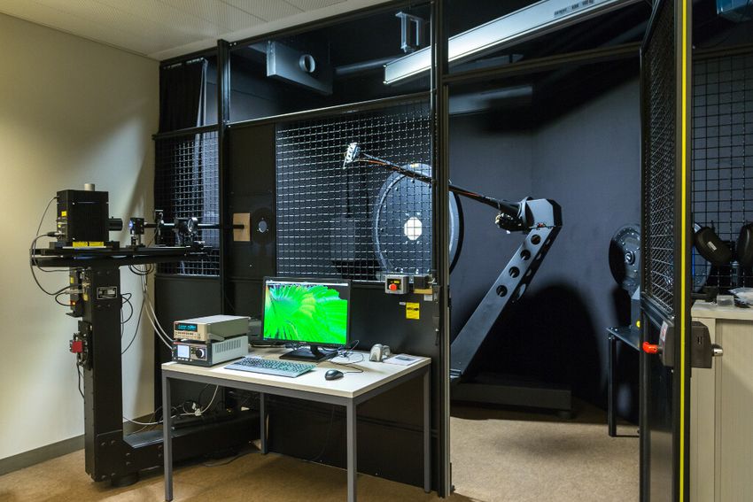
P��� ������� �� P���������

7   “Everything the Light Touches” – Rendering The Lion King                                                                             24

8   Introduction of GPU production path tracing at Digital Domain                                                                        25
    8.1 Introduction to rendering at Digital Domain . . . . . . . . . .      .   .   .   .   .   .   .   .   .   .   .   .   .   .   .   25
    8.2 Evolution not Revolution . . . . . . . . . . . . . . . . . . . .     .   .   .   .   .   .   .   .   .   .   .   .   .   .   .   25
         8.2.1 Testing in the Sandbox . . . . . . . . . . . . . . . . .      .   .   .   .   .   .   .   .   .   .   .   .   .   .   .   25
         8.2.2 Animation Renders . . . . . . . . . . . . . . . . . . .       .   .   .   .   .   .   .   .   .   .   .   .   .   .   .   25
         8.2.3 Immediate benefits . . . . . . . . . . . . . . . . . . .      .   .   .   .   .   .   .   .   .   .   .   .   .   .   .   26
    8.3 Software Challenges . . . . . . . . . . . . . . . . . . . . . . .    .   .   .   .   .   .   .   .   .   .   .   .   .   .   .   27
         8.3.1 Basic Requirements . . . . . . . . . . . . . . . . . . .      .   .   .   .   .   .   .   .   .   .   .   .   .   .   .   27
         8.3.2 Advanced Development . . . . . . . . . . . . . . . . .        .   .   .   .   .   .   .   .   .   .   .   .   .   .   .   27
    8.4 Hardware . . . . . . . . . . . . . . . . . . . . . . . . . . . . .   .   .   .   .   .   .   .   .   .   .   .   .   .   .   .   28
         8.4.1 Rendering with artists’ desktops . . . . . . . . . . . . .    .   .   .   .   .   .   .   .   .   .   .   .   .   .   .   28
         8.4.2 Building a GPU Render farm . . . . . . . . . . . . . .        .   .   .   .   .   .   .   .   .   .   .   .   .   .   .   28
    8.5 Production Lessons . . . . . . . . . . . . . . . . . . . . . . .     .   .   .   .   .   .   .   .   .   .   .   .   .   .   .   29
         8.5.1 The Learning Curve . . . . . . . . . . . . . . . . . . .      .   .   .   .   .   .   .   .   .   .   .   .   .   .   .   29
         8.5.2 Being Prepared Earlier . . . . . . . . . . . . . . . . .      .   .   .   .   .   .   .   .   .   .   .   .   .   .   .   30
         8.5.3 Setting a Look . . . . . . . . . . . . . . . . . . . . . .    .   .   .   .   .   .   .   .   .   .   .   .   .   .   .   30
         8.5.4 Possible confusion . . . . . . . . . . . . . . . . . . . .    .   .   .   .   .   .   .   .   .   .   .   .   .   .   .   30
    8.6 Benefits of GPUs for other VFX processes . . . . . . . . . . . .     .   .   .   .   .   .   .   .   .   .   .   .   .   .   .   31
    8.7 Conclusion . . . . . . . . . . . . . . . . . . . . . . . . . . . .   .   .   .   .   .   .   .   .   .   .   .   .   .   .   .   31
    8.8 Acknowledgements . . . . . . . . . . . . . . . . . . . . . . . .     .   .   .   .   .   .   .   .   .   .   .   .   .   .   .   31

SIGGRAPH 2019               Course Notes: Path tracing in Production — Part 2                                                Page 2 / 32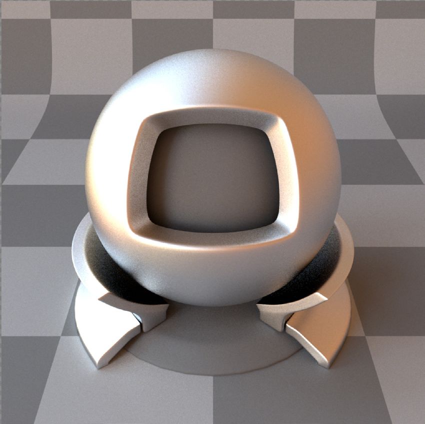
P��� ������� �� P���������

1    Objectives
In the past few years the movie industry has switched over from stochastic rasterisation approaches to using
physically based light transport simulation: path tracing in production has become ubiquitous across studios.
The new approach came with undisputed advantages such as consistent lighting, progressive previews, and
fresh code bases. But also abandoning 30 years of experience meant some hard cuts affecting all stages such as
lighting, look development, geometric modelling, scene description formats, the way we schedule for multi-
threading, just to name a few. This means there is a rich set of people involved and as an expert in one of the
aspects it is easy to lose track of the big picture.
     This is part II of a full-day course, and it focuses on a number of case studies from recent productions at
different facilities, as well as recent development in material modeling and capturing. The presenters will will
showcase practical efforts from recent shows spanning the range from photoreal to feature animation work,
pointing out unexpected challenges encountered in new shows and unsolved problems as well as room for
future work wherever appropriate.
     This complements part I of the course, where context was provided for everybody interested in under-
standing the challenges behind writing renderers intended for movie production work, with a focus on new
students and academic researchers. On the other side we will lay a solid mathematical foundation to develop
new ideas to solve problems in this context.

SIGGRAPH 2019                Course Notes: Path tracing in Production — Part 2                       Page 3 / 32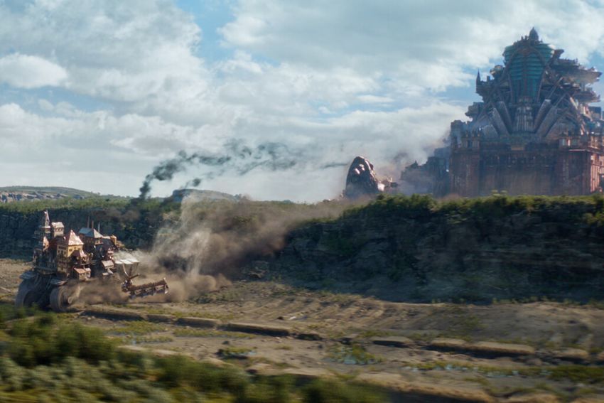
P��� ������� �� P���������

2     Syllabus
2.1   14:00 — Opening statement
      (Luca Fascione, 15 min)
A short introduction to the topics in this session and to our speakers.

2.2    14:15 — Capturing and rendering the world of materials
       (Wenzel Jakob, 30 min)
One of the key ingredients of any realistic rendering system is a description of the way in which light interacts
with objects, typically modeled via the Bidirectional Reflectance Distribution Function (BRDF). Unfortunately,
real-world BRDF data remains extremely scarce due to the difficulty of acquiring it: a BRDF measurement
requires scanning a four-dimensional domain at high resolution–an infeasibly time-consuming process.
     In this talk,Wenzel will showcase the ongoing work at EPFL on assembling a large library of materials in-
cluding metals, fabrics and organic substances like wood or plant leaves. The key idea to work around the curse
of dimensionality is an adaptive parameterization, which automatically warps the 4D space so that most of the
volume maps to “interesting” regions. Starting with a review of BRDF models and microfacet theory, Wenzel
will explain the new model, as well as the optical measurement apparatus used to conduct the measurements.

2.3    14:45 — Production quality materials
       (Andrea Weidlich, 30 min)
Recent film productions like Mortal Engines or Alita: Battle Angle exhibit an unprecedented visual richness that
was unthinkable ten years ago. One key component to achieve this is a flexible but expressive material system
that is capable of reproducing the complexity of real-world materials but is still simple enough so that it can
be used on a large scale. Andrea will talk about material modeling in a production path tracer in general and
the constraints that come about when artistically driven decisions meet a physically plausible world. She will
demonstrate how a modern layer-based material system as it can be found in Weta Digital’s in-house renderer
Manuka influences design and look development decisions, and give examples of how it is used in production.

2.4    15:15 — Break (15 min)
2.5    15:30 — “Everything the Light Touches” – Rendering The Lion King
       (Rob Pieké, 30 min)
Not long after the success of Disney’s The Jungle Book, MPC Film began work on the retelling of another Disney
classic: The Lion King. The mandate for this project was to bring realistic environments and documentary-style
cinematography to the screen, requiring improvements across the board to our rendering-related technology,
workflows and pipelines. In this talk, Rob will outline some of the changes to MPC’s fur rendering, improve-
ments in outdoor environment rendering efficiency, advancements to deep image workflows and more.

2.6    16:00 — Introduction to GPU production path tracing at Digital Domain
       (Hanzhi Tang, 30 min)
Starting in 2016 Digital Domain has been testing GPU rendering, trying to see how it would integrate into the
production rendering pipeline smoothly. Starting from initial qualitative tests to widespread use on Avengers:
Infinity War to final production renders on Captain Marvel, Digital Domain built a robust GPU rendering option
that sits alongside the main CPU rendering pipeline. Hanzhi Tang will present the development challenges of
both hardware and software that were encountered in this implementation of this new renderer.

2.7    16:30 — Q&A with all presenters (15 min)

SIGGRAPH 2019                Course Notes: Path tracing in Production — Part 2                       Page 4 / 32
P��� ������� �� P���������

3     Organizers
3.1   Luca Fascione, Weta Digital
                   Luca Fascione is Head of Technology and Research at Weta Digital where he oversees
                   Weta’s core R&D efforts including Simulation and Rendering Research, Software Engi-
                   neering and Production Engineering. Luca architected Weta Digital’s next-generation
                   proprietary renderer, Manuka with Johannes Hanika. Luca joined Weta Digital in 2004
                   and has also worked for Pixar Animation Studios. The rendering group’s software, includ-
                   ing PantaRay and Manuka, has been supporting the realization of large scale productions
                   such as Avatar, The Adventures of Tintin, the Planet of the Apes films and the Hobbit trilogy.
                   He has recently received an Academy Award for his contributions to the development
                   of the facial motion capture system in use at the studio since Avatar.

3.2    Johannes Hanika, Weta Digital
                   Johannes Hanika received his PhD in media informatics from Ulm University in 2011.
                   After that he worked as a researcher for Weta Digital in Wellington, New Zealand. There
                   he was co-architect of Manuka, Weta Digital’s physically-based spectral renderer. Since
                   2013 he is located in Germany and works as a post-doctoral fellow at the Karlsruhe Insti-
                   tute of Technology with emphasis on light transport simulation, continuing research for
                   Weta Digital part-time. In 2009, Johannes founded the darktable open source project,
                   a workflow tool for ��� photography, and he has a movie credit for Abraham Lincoln:
                   Vampire Hunter.

4     Presenters
4.1   Wenzel Jakob, EPFL
                   Wenzel Jakob is an assistant professor at EPFL’s School of Computer and Communication
                   Sciences, where he leads the Realistic Graphics Lab (https://rgl.epfl.ch/). His research
                   interests revolve around material appearance modeling, rendering algorithms, and the
                   high-dimensional geometry of light paths. Wenzel Jakob is also the lead developer of
                   the Mitsuba renderer, a research-oriented rendering system, and one of the authors of
                   the third edition of the book Physically Based Rendering: From Theory To Implementation.
                   (http://pbrt.org/)

4.2    Andrea Weidlich, Weta Digital
                   Andrea Weidlich is a Senior Researcher at Weta Digital where she is responsible for the
                   material system attached to Weta’s proprietary physically-based renderer, Manuka. An-
                   drea grew up in Vienna,Austria, where she studied technical computer science, and later
                   focused on computer graphics. After finishing her Ph.D.for predicting the appearance of
                   crystals she switched to the private sector and moved to Munich to work for the automo-
                   tive industry. Her continuing work on Manuka allows Weta to produce highly complex
                   images with unprecedented fidelity. Her main research areas are appearance modeling
                   and material prototyping. Andrea holds a Master of Arts in Applied Media from the
                   University of Applied Arts, Vienna and a Ph.D. in Computer Science from the Vienna Uni-
                   versity of Technology.

SIGGRAPH 2019             Course Notes: Path tracing in Production — Part 2                          Page 5 / 32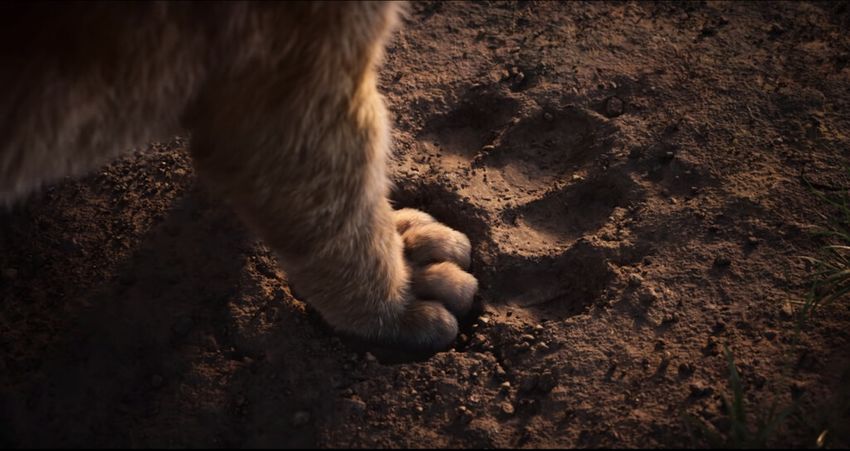
P��� ������� �� P���������

4.3   Rob Pieké, MPC
                 Rob Pieké is the Head of New Technology at MPC in the heart of London. Having re-
                 cently celebrated his tenth year with the company, Rob has been involved in the devel-
                 opment of custom artist tools for dozens of films, from Harry Potter to Guardians of the
                 Galaxy and, most recently, The Jungle Book. Rob started programming in ����� as a kid,
                 and went on to get a degree in Computer Engineering from the University of Waterloo in
                 Canada. With his passion for computer graphics — rendering and physical simulation
                 in particular — the visual effects industry caught Rob’s eye quickly, and he’s never looked
                 back since.

4.4   Hanzhi Tang, Digital Domain
                 Hanzhi Tang is a Digital Effects Supervisor and Head of Lighting at Digital Domain. He
                 received an MSc in Physics from Imperial College, University of London and has been
                 with Digital Domain for 16 years working with many different production renderers on
                 23 feature films. He also recently became a member of the Academy of Motion Picture
                 Arts and Sciences and has previously been a Visual Effects Society Awards nominee. He
                 has most recently completed visual effects on Captain Marvel from Marvel Studios.

SIGGRAPH 2019           Course Notes: Path tracing in Production — Part 2                       Page 6 / 32
P��� ������� �� P���������

Figure 1: Spectral rendering of isotropic and anisotropic materials acquired from real-world samples using our method; insets show
corresponding reflectance spectra. We measured these ����s using a motorized gonio-photometer, leveraging our novel adaptive
parameterization to simultaneously handle ���� acquisition, storage, and efficient Monte Carlo sample generation during render-
ing. Our representation requires 16 KiB of storage per spectral sample for isotropic materials and 544 KiB per spectral sample for
anisotropic specimens.

5       Capturing and rendering the world of materials
        W����� J����, EPFL
        Joint work with J������� D����

One of the key ingredients of any realistic rendering system is a description of the way in which light interacts
with objects, typically modeled via the Bidirectional Reflectance Distribution Function (����). Unfortunately,
real-world ���� data remains extremely scarce due to the difficulty of acquiring it it: a ���� measurement
requires scanning a five-dimensional domain at high resolution—–an infeasibly time-consuming process.
    In this talk, I’ll showcase our ongoing work on assembling a large library of materials including metals,
fabrics, organic substances like wood or plant leaves, etc. The key idea to work around the curse of dimen-
sionality is an adaptive parameterization, which automatically warps the 4D space so that most of the volume
maps to “interesting” regions. Starting with a review of ���� models and microfacet theory, I’ll explain the
new model, as well as the optical measurement apparatus that we used to conduct the measurements1 .

5.1     Introduction
Physically based rendering algorithms simulate real-world appearance by means of an intricate simulation of
the interaction of light and matter. Scattering by surfaces denotes the most important type of interaction, and
the physics of this process are typically encoded in a quantity known as the bidirectional reflectance distribu-
tion function (����). High-fidelity ���� models thus constitute a crucial ingredient to any type of realistic
rendering. In this work, we are interested in acquiring real-world ���� data and propose a practical ���� rep-
resentation that simultaneously serves as a mechanism for acquisition, storage and sample generation within
rendering software.
    1
     This document is an informal writeup of the paper “An Adaptive Parameterization for Efficient Material Acquisition and Ren-
dering” by Jonathan Dupuy and Wenzel Jakob published at SIGGRAPH Asia 2018. For a detailed technical description, please refer
to the original paper. Our database and an open source reference implementation is available at https://rgl.epfl.ch/materials

SIGGRAPH 2019                     Course Notes: Path tracing in Production — Part 2                                  Page 7 / 32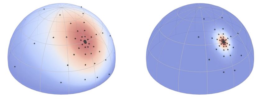
P��� ������� �� P���������

                                                    Observer

                                                                       Light source

                                                     Material sample

     Given illumination arriving from a specific direction, the ���� specifies the directional profile of light
scattered by a surface. The availability of such measurements is important not only because they improve re-
alism, but also because they serve as validation against theoretical models that help advance our understanding
of light-material interactions. For instance, the ���� database [Matusik et al., 2003] has served as inspiration
and validation of numerous ���� models over the last fifteen years.

Challenges. Being dependent on two directions and wavelength, the ���� is a five-dimensional quantity.
This makes it extremely costly to discretize or measure at sufficiently high resolution due to the curse of di-
mensionality. For instance, suppose that a material is to be measured with a (still relatively coarse) 1002 regular
grid for both incident and outgoing direction, and that the used device is able to perform one measurement
per second that captures all wavelengths at once.

These assumptions are in fact fairly optimistic–even so, the measurement would require in excess of three
years! Because of these difficulties, existing measurements have been limited to coarse resolutions in either or
both the directional and spectral domains.
    Our objective is to significantly shorten the acquisition time to make this process more practical (on the
order of a few hours for isotropic samples, and a few days for anisotropic samples). To our knowledge, we are
the fist to provide high resolution ���� data that includes spectral information and anisotropy.

Prior work. Although we can’t completely avoid the curse of dimensionality, there are techniques that can
be applied to mitigate its effects by placing samples in a more informed manner. For instance, parameteriza-
tions built around the half-angle [Rusinkiewicz, 1998] can be used to naturally align the discretization with
the direction of specular reflection, allowing for high-quality acquisition with fewer samples.

SIGGRAPH 2019                 Course Notes: Path tracing in Production — Part 2                        Page 8 / 32
P��� ������� �� P���������
It also seems intuitive that different sampling patterns should be used depending on the material properties
(e.g. for diffuse, mirror-like, or anisotropic materials). However, current parameterization approaches do not
possess this type of adaptivity–the parameterization is always the same.
The work that is most relevant to this project is the technique described in [Matusik et al., 2003], which
was used to measure a collection of 100 isotropic ����s known as the ���� database. Acquisition using this
approach involves photographing a spherical material sample from a static camera for a number of lighting
directions (the image below is taken from the original paper and shows the measurement setup).
The resulting data is then stored using the Rusienkiewicz [Rusinkiewicz, 1998] parameterization. The use of
spherical samples significantly reduces the measurement time, since each photograph provides observation
of a large set of normal vectors, corresponding to a two-dimensional slice through the ����. On the flipside,
this approach suffers from a number of drawbacks that we aim to address in our work
• Photographing shiny spherical targets illuminated with collimated illumination is not unlike taking
pictures of the sun–the images have an extremely large dynamic range and will be contaminated with
lens flare, which affects the contents of adjacent pixels. We believe that this is the source of a number of
artifacts present in the original dataset [Burley, 2012].
• Due to the fixed parameterization, the sampling pattern used is the always identical regardless of the
material being scanned. This means that certain materials, for which the sampling density is unsuitable
(e.g. very narrowly peaked ones) will suffer from significant errors.
• It is very easy to obtain metallic spheres of various sizes, and some manufacturers of plastic spheres can
also be found. Spheres can furthermore be spray-painted to enlarge the space of material somewhat.
Beyond this, we have found it extremely challenging to procure suitable spherical samples of materials
(e.g. cloth, wood, etc.). Any measurement technique that uses this approach is thus confronted with
an inherent bias towards materials (mostly paints) that are available in spherical form. Our goal is to
provide a richer set of materials including cloth, organic materials (e.g. plant leaves) and anisotropically
brushed metals.
• The database only contains isotropic materials, while many materials are in fact anisotropic. The reason
for this is that many surfaces are processed (e.g. polished) or created by tools that operate in a directional
manner (turning, milling, lathing, etc.).
• The representation does not provide a natural importance sampling method and must be combined
with other techniques that compute auxiliary data structures to be usable in a renderer. Our goal is the
design of a single representation that is simultaneously usable for acquisition, storage, and rendering.
• A meta-issue of this dataset is the lack of information on what parts of the data are“real”, and what parts
are extrapolated or post-processed. In particular, an issue faced by any ���� measurement device is
that certain configurations are unobservable due to hardware limitations and must be approximated
using an interpolant. We preserve the raw data of all measurement sessions to this problem.
5.2 Adaptive parameterization
Our measurement technique relies on a sampling pattern that adapts to the material being acquired. For
instance, rough materials are sampled at a broad set of directions (left), while narrowly peaked materials use
SIGGRAPH 2019 Course Notes: Path tracing in Production — Part 2 Page 9 / 32P��� ������� �� P���������
a more compact pattern matching the material’s behavior. Anisotropic materials (not shown here) such as
brushed metals use a suitably distorted anisotropic pattern.
Determining a good sampling pattern initially appears like a classic chicken-and-egg problem: we must al-
ready have acquired the material to make an informed decision on where samples should be placed. Fortu-
nately, it turns out that we can use leverage the rich body of research on scattering from rough surfaces (in
particular, microfacet theory) to resolve this conundrum.
5.2.1 Retro-reflection
Our approach is based on the observation that retro-reflection configurations (i.e. where ωi = ωo ) are com-
parably easy to measure. Acquisition of such configurations for a single wavelengths unproblematic, since the
domain is only two-dimensional (i.e., relatively unaffected by the curse of dimensionality). At the same time,
retro-reflection encodes helpful information that characterizes the material behavior. For instance, consider
the following retro-reflection plots of three different material classes.
Our objective is to turn this cue into a suitable sampling pattern.
To do so, we shall temporarily introduce an assumption: what if the material being measured perfectly
satisfied the predictions of microfacet theory? In this case, the retro-reflective response of the ���� f is pro-
portional to
D(ω)
f (ω, ω) ∝ (1)
σ(ω) cos θ
where D is the material’s microfacet distribution and σ is the projected area of the microfacet surface (which
also depends on D). There is thus a direct relationship between retro-reflection and microfacet distribution,
and we show in the paper that D can easily be reconstructed from such measurements by finding the largest
eigenvector of a matrix. In other words: if the material indeed satisfies microfacet theory, we know everything
only from a single capture of the retro-reflective response. We will now briefly turn to another operation,
namely importance sampling.
5.2.2 Inverse transform sampling
Recall the canonical mechanism for designing importance sampling strategies, known as inverse transform
sampling: starting from a density p(x), we first create the cumulative distribution function
x
P(x) = ∫ p(x′ ) dx′ , (2)
−∞
and its inverse P −1 is then used to map transform uniformly distributed variates on the interval [0, 1]. By
construction, this yields samples with the right distribution.
SIGGRAPH 2019 Course Notes: Path tracing in Production — Part 2 Page 10 / 32P��� ������� �� P���������
Another view of inverse transform sampling is that it creates a parameterization of a domain that expands and
contracts space in just the right way so that different parts receive a volume proportional to their integrated
density.
Virtually all importance sampling techniques–including those of microfacet ���� models–are based on
inverse transform sampling and thus can also serve as parameterizations if supplied with non-random inputs.
5.2.3 Putting all together
These, then, constitute the overall building blocks of our approach:
(i) Starting with a retro-reflection measurement, we compute the properties (i.e. D, σ) of a hypothetical
microfacet material that behaves identically.
(ii) Next, we process D to generate tables for the inverse transform sampling technique.
(iii) Finally, we use the sampling technique as a parameterization to warp the ���� into a well-behaved
function that is easy to sample using a regular grid (which turns into a high-quality sampling pattern
after passing through the parameterization).
Warp 1 Warp 2 Warp 3 Capture Weight
1.0 1.0
Acqire
0.5 0.5
)
(4D
0.0 0.0
F
0.0 0.5 1.0 0.0 0.5 1.0
Regular grid D
VN
Warp 1 Warp 2 Warp 3 Warp 4 Integrate
1.0 1.0 1.0
Sample
Starting from a regular grid, the above image visualizes the involved operations, which are the composition
0.5 0.5 0.5
of a sequence of invertible
0.0
nc
e(
)
4Doperations g1 (inverse
(4D
0.0 ) transform mapping), g2 (square-to-sphere mapping), and g3
0.0
DF
0.0 0.5 1.0 0.0 0.5 1.0
ina
0.0 0.5 1.0
Uniform samples
m VN
(specular reflection from
Lu a microfacet). Also note that this sequence is not just useful for acquisition–it also
Inverse Warp 1 Inverse Warp 2 Inverse Warp 3 Interpolate
enables efficient importance sampling at render time.
Evaluate
1.0 1.0
An important aspect of our previous assumption of microfacet theory-like behavior is that it is merely
0.5 0.5
)
) 5D
used to generate a parameterization–no other part of our approach DF
(4D depends on peit.
0.0
0.0 0.5
ctr
a ( This means that we are
1.0
0.0
0.0 0.5 1.0
360nm 1000nm
VN S
also able to acquire functions that are in clear violation of this assumption, although this will manifest itself
in interpolants that are less smooth and hence require a denser discretizations.
We briefly outline two additional important technical details–for further details, please refer to the paper:
1. Different microfacet importance sampling schemes exist, including ones that produce lower variance
in traditional Monte Carlo rendering applications. Interestingly, a superior sampling scheme also tends
to produce smoother interpolants in our application. We sample distribution of visible normals intro-
duced in [Heitz and d’Eon, 2014] for this reason.
2. When a density function is re-parameterized on a different domain (e.g. from Euclidean to polar coor-
dinates), we must normally multiply by the determinant of the Jacobian to obtain a valid density that
accounts for the expansion and contraction of the underlying mapping. In our application, we also
observed that it is beneficial to multiply ���� measurements by the combined Jacobian of the above
functions g1 to g3 , which yields an even smoother function that can stored at fairly low resolutions (e.g.
32x32).
5.3 Hardware
Our acquisition pipeline relies on a modified PAB pgII [PAB, 2018] gonio-photometer, which acquires spectral
���� samples at a rate of approximately 0.5-1 samples per second.
SIGGRAPH 2019 Course Notes: Path tracing in Production — Part 2 Page 11 / 32P��� ������� �� P���������
This device illuminates a flat vertically mounted sample from a light source that is mounted one of two sta-
tionary rails (we use both during acquisition). To change the incident light direction, the motorized sample
mount rotates around the vertical axis and the normal direction of the sample. A sensor head mounted on
a motorized two-axis arm measures the illumination scattered by the sample. We use a mounted Z���� fiber
spectrometer to capture dense (∼ 3nm spacing) spectral curves covering the 360-1000nm range.
The machine has two “dead spots” that cannot be measured with the combination of sensor arm and light
source: first, the sensor arm cannot view the sample from straight below, since this space is occupied by the
pedestal holding the sample mount. Second, shadowing becomes unavoidable when the sensor is within ap-
proximately 3 degrees of the beam, making retro-reflection measurements impossible.
The former is unproblematic and can be reconstructed without problems. However, the latter is a signif-
icant impediment, since the method presented so far heavily relies on the ability to perform an initial retro-
reflection measurement. We work around this limitation by using two separate illumination and measurement
paths shown below:
DPSS laser Kinematic mirrors (2x) Sample holder
Beamsplitter Sensor head
Photodiode
Electronic shutter
Beam dump 50mm
plano-convex Beamsplitter
Beam expander
Beam expander Focusing
(250mm plano-convex,
lens (300mm) Beam dump
25mm bi-concave)
Electronic
shutter
Collimation lens Faraday isolator
Pinhole Sample
(1mm)
Faraday Photodiode
isolator
Pinhole Electronic shutter
Alignment
mirrors
Focusing lens
Xenon arc light source
DPSS laser Xenon arc light source
(532nm, 40mW) (XBO 150W/CR OFR)
In the first phase, we rotate the sensor arm in a configuration so as to avoid blocking any lighting from the
laser onto the sample, and a laser illuminates the sample through a beamsplitter. Retro-reflected illumination
from the sample reaches the same beamsplitter and is reflected onto a small photodiode, whose current we
measure. The second measurement stage uses a broadband xenon arc light source along with the spectrometer
along with the normal spectral sensor on the sensor arm.
5.4 Database
We’re currently in the process of acquiring a large database of materials using the presented technique. Our
objective is that this database eventually grows to many hundreds of entries that sample the manifold of nat-
ural and man-made. Outside help is welcomed during this process: if you have interesting samples, we’d love
to measure them!
Please see https://rgl.epfl.ch/materials for a web interface of what was acquired thus far. Scans on this
page can be interactively viewed and analyzed using the Tekari viewer created by Benoît Ruiz, which runs
using WebGL and WebAssembly. For this, simply click on any material to expand the entry, and then push the
Interactive viewer button. We’ve also released a reference ���� implementation, which provides the standard
operations needed by most modern rendering systems: ���� evaluation, sampling, and a routine to query
the underlying probability density. The repository also contains a plugin for the Mitsuba renderer and Python
SIGGRAPH 2019 Course Notes: Path tracing in Production — Part 2 Page 12 / 32P��� ������� �� P���������
code to load the data files into NumPy, which is useful for visualization and systematic analysis of the database
contents. All resources are linked from the material database page.
We briefly discuss two visualizations that are shown on ���� database page: the below image shows an
��� rendition of what was measured by the spectrometer using our parameterization. Note that the data
typically has extremely high-dynamic range, hence some detail in the black may simply be invisible. Red
pixels correspond to wasted space of the discretization. The black column on the left is a region that could not
be measured.
This following plot contains the same data, but after post-processing. The black regions on the left were filled
in, and the data was scaled by the Jacobian of the parameterization (see the paper for details). This has the
effect of making the representation significantly easier to interpolate. The bottom row shows spectral curves
in the 360-1000nm range corresponding to the row above.
Since our acquisition device captures full color spectra,we’ve so far scanned many materials with wave-optically
interesting behavior (which often have oscillatory reflectance spectra). Figure 2 contains a few selected visu-
alizations.
5.5 Conclusion
We have presented the first adaptive ���� parameterization that simultaneously targets acquisition, storage,
and rendering. We used our method to introduce the first set of spectral ���� measurements that contain
both anisotropy and high frequency behavior. Our dataset contains many materials with spectrally interesting
behavior (multiple types of iridescent, opalescent, and color-changing paints).
We find that the availability of spectral ���� datasets is timely: as of 2018, major industrial systems render
in the spectral domain (e.g. Maxwell, W��� D������’s Manuka renderer), and two major open source renderers,
PBRT and Mitsuba, are presently being redesigned for full-spectral rendering [Pharr and Jakob, 2017]. We
believe that access to a comprehensive spectral dataset will enable future advances in the area of material
modeling.
Going forward, we are also interested in using our technique to model materials with spatial variation–this
involves the additional challenge that an ideal sampling pattern is now likely different for each spatial location,
and a compromise must thus be reached to turn this into a practical measurement procedure. Furthermore,
storage becomes prohibitive and compression strategies are likely needed even during a measurement. The
hardware of our gonio-photometer was recently extended, allowing us to mount high-resolution ��� and
���� cameras onto the sensor arm, and we look forward to facing these new challenges in the future.
References
Brent Burley. 2012. Physically-based shading at Disney. In ACM SIGGRAPH 2012 Courses (SIGGRAPH ’12).
ACM, New York, NY, USA.
SIGGRAPH 2019 Course Notes: Path tracing in Production — Part 2 Page 13 / 32P��� ������� �� P���������
6 aurora-white 19 ibiza-sunset 31 silk-blue
Description: TeckWrap vinyl wrapping �lm ("Aurora White DCH02") Description: Car wrap material (Teckwrap Ibiza Sunset RD02) Description: Blue car wrap (Teckwrap Silk Blue VCH502N)
Renderings Renderings Renderings
u�zi.exr wells.exr topanga.exr u�zi.exr wells.exr topanga.exr u�zi.exr wells.exr topanga.exr
Plots Plots Plots
Sample Locations Sample Locations Sample Locations
Slices Slices Slices
measured
measured
measured
weighted
weighted
weighted
�lled
�lled
�lled
spectra
spectra
spectra
7 20 32
20 iridescent-�ake-paint2 29 nothern-aurora 26 l3-metallic
Description: Iridescent car paint with �akes Description: Car wrap material (Teckwrap Nothern Aurora RD05) Description: Metallic paint from L3 robot (from "Solo: A Star Wars Story", provided by ILM)
Renderings Renderings Renderings
u�zi.exr wells.exr topanga.exr u�zi.exr wells.exr topanga.exr u�zi.exr wells.exr topanga.exr
Plots Plots Plots
Sample Locations Sample Locations Sample Locations
Slices Slices Slices
measured
measured
measured
weighted
weighted
weighted
�lled
�lled
�lled
spectra
spectra
spectra
21 30 27
Figure 2: Visualizations of selected materials from our database.
Eric Heitz and Eugene d’Eon. 2014. Importance Sampling Microfacet-Based BSDFs using the Distribution of
Visible Normals. In Computer Graphics Forum, Vol. 33. 103–112.
Wojciech Matusik, Hanspeter Pfister, Matt Brand, and Leonard McMillan. 2003. A Data-Driven Reflectance
Model. ACM Trans. Graph. 22, 3 (July 2003), 759–769.
PAB. 2018. pab advanced technologies Ltd. http://www.pab.eu. Accessed: 2018-01-09.
Matt Pharr and Wenzel Jakob. 2017. personal communication.
Szymon M Rusinkiewicz. 1998. A New Change of Variables for Efficient BRDF Representation. In Rendering
Techniques ’98. Springer, 11–22.
SIGGRAPH 2019 Course Notes: Path tracing in Production — Part 2 Page 14 / 32P��� ������� �� P���������
6 Material Modeling in a Modern Production Renderer
A����� W�������, Weta Digital
6.1 Motivation
Modern computer graphics have reached astonishing levels of visual realism and artistic expression. As our
technological abilities have progressed, several distinct sub-fields, each with its unique technical challenges
and goals, have emerged within the discipline. Examples are non-photorealistic rendering, scientific visuali-
sation or production techniques geared for the entertainment industry.
During the last ten years, physically based rendering managed to gain so much importance that nowa-
days it can be regarded robust enough for all application domains that it might be considered for. Significant
progress has been made towards shading techniques under the constraints of such rendering systems. In part
this is because rendering algorithms have advanced so far that we can spend more time generating complex
materials. And while for the longest time it was acceptable to limit the creativity of a user to a very small subset
of materials which were put together in an uber-shader, more and more applications provide layered models,
albeit with varying degree of physical correctness.
The two big advantages of layered models are that they are physically based (if not entirely physically
correct in the narrow sense of the word because of the approximations that are still introduced into the evalu-
ation) and therefore produce feasible looking results, and are intuitive to use at comparably low computational
costs. Getting accustomed to shade with a layered approach instead of using single un-layered models meant
a paradigm shift in the workflow and a new way of thinking. And while ten years ago layered shading models
were still a niche product and the general agreement was that one can either have physically correctness or
artistic freedom, physically based shading models are nowadays a basic component not only in expensive high
quality rendering, but also in many realtime applications.
This section of the course will review the development of the material system in Manuka, the production
path tracer in use at W��� D������, used on movies like Mortal Engines (2018) or Alita: Battle Angel (2019). We
will discuss the design decisions we had to make and how they affect the way we work with materials in our
production environment.
6.2 Design Ideas
With hundreds and hundreds of different assets and palettes in a single movie, a modern material systems in
a production path tracer needs to be able to fulfill several requirements
• Flexibility. Different characters require different visual complexity, and a material system must be ver-
satile enough to adapt to different production requirements. Within one scene we have not only hero
characters but also background characters, environments and atmospheric effects. While the majority
of our characters are realistic, we also need to be able to model a more cartoony look-and-feel. We do
not want to limit ourselves to one particular class of ����s (such as having only microfacet models)
and want to have the flexibility to adapt the system to evolving requirements.
• Storage. Solutions for realistic appearance models often demand heavy pre-computation. Since we rely
on visual complexity, we heavily make use of textures and cannot incur long pre-computation times
nor excessive per-vertex or per-asset storage costs.
• Artistic Freedom. While materials in a path tracer have to fulfill certain physical requirements like energy
conservation and Helmholz reciprocity, their usage is not bound to be physically correct. We frequently
have to deal with appearances that do not exist in reality and even more often have to tweak materials
based on artistic decisions. While we do aim for physical plausibility, we need to be prepared to give
users the possibility to break reality.
SIGGRAPH 2019 Course Notes: Path tracing in Production — Part 2 Page 15 / 32P��� ������� �� P���������
• Computation Time. Since we have only a certain time budget to render a movie, computation time is an
important factor. We need to be able to turn certain effects on and off based on budget. Sampling must
be efficient.
6.3 Manuka’s Material System
W��� D������’s proprietary in-house renderer Manuka [Fascione et al., 2018] is a spectral path tracer that
comes with a powerful material system. It was first used in production on the movie Dawn of the Planet of the
Apes (2014) and back then had already the same basic components we use today. The key design decision was
to aim for the most flexible material system possible. Instead of implementing just one powerful uber-shader,
Manuka supports a layer-based material system that lets the user combine arbitrary ����s and assemble them
into a material stack.
Currently we support over a hundred different ����s which are all layer-able. These ����s include a
variety of different appearance descriptions, some have an academic background and were developed inside
and outside of the rendering community, others were built in-house. We differ between several ���� classes:
����s reflect only, ����s only transmit, ����s which scatter in both hemispheres, �����s for curves and
���s for emission. All ����s are flagged according to their type and during light transport we make use of
this information to make sampling and computations more efficient.
Regardless of their type, all ����s need to implement the same interface. Apart from the functions one
would expect in a path tracer, such as Sample(), Eval() and Pdf(), we have functions which inform the renderer
about ����-specific information like mean directions, ���s and reflectance, average roughness or energy dis-
tribution. All ����s can be versioned in order to support older and newer versions of the same ���� int he
same process, to facilitate shader and model evolution at different paces for different assets.
6.3.1 Shade-before-Hit vs. Shade-on-Hit
Different from the other production renderers we are aware of, Manuka has a shading architecture which we
called shade-before-hit [Fascione et al., 2018], where instead of evaluating shaders upon a ray-hit event, most
of the shading computation happens before ray tracing starts. This unique design decision comes with ad-
vantages and disadvantages. Since we do not have to evaluate shaders on the fly, we avoid having to execute
expensive texture reads upon ray-hit, which can cause difficult to mitigate bottle-necks due to lack of locality
of reference inherent in the path tracing algorithm. Therefore, our architecture allows production shading
networks to become much larger and more detailed than usual production shader networks, and in fact they
commonly have dozens of texture reads per ����. Consequently we can achieve much higher visual com-
plexity.
On the other hand, our shading has to be completely view-independent and during light transport we
cannot access material information of neighbouring pixels. Instead, everything needs to be done inside the
material system. The shaders role is to leave on the micropolygon vertices the ���� parameters and the weights
of ����s and layers, as well as the layout of the layer-stack.
Compression of the data is a huge help, since everything is stored on the micropolygon grids. We have
observed that 8-bit tends to be enough for most colour data, such as albedo values, however roughness and
similar data is stored in 16-bit to avoid banding artifacts.
6.3.2 Filtering Techniques
While it is true that Manuka’s architecture achieves more complex materials at a lower cost during runtime,
this obviously comes with a cost in memory. Our RenderMan heritage implies that final shading quality is
determined by the shading rate. For this reason, filtering techniques become more important, as we store the
data on the vertices and cannot access textures during light transport. For non-linear data such as normals,
filtering is not straightforward. Techniques like ���� mapping [Olano and Baker, 2010] or [Han et al., 2007]
become essential to keep the look of an asset consistent between close-up and distant shots. Loss of surface
detail has to be recovered with techniques like [Yan et al., 2014] or [Jakob et al., 2014].
SIGGRAPH 2019 Course Notes: Path tracing in Production — Part 2 Page 16 / 32P��� ������� �� P���������
However, not all data can be filtered easily. A problematic example is interference data or blackbody tem-
perature. When we pass in numerical data that is converted into colour through strongly non-linear relations,
the interpolate-then-filter and filter-then-interpolate approaches have a high chance of producing markedly
different results. These filtering techniques are implemented upstream of Manuka.
6.3.3 Spectral Input Data
Manuka is a spectral renderer, and all ����s compute their quantities in a spectrally-dependent manner. How-
ever, the majority of our input data is in some ��� space, since artist workflows and software at present is only
available to us this way. During rendering we spectrally lift the data (see Section 1.4.2 in the first part of this
course for further details). This results in the interesting problem that, since there is no unique correspon-
dence between a single spectrum and a specific ��� value, the spectra we generate are somewhat arbitrary
and not exactly the one from the photographed reference asset. This far it seems to us that the many of our
use cases are somewhat forgiving and that the practical simplicity of an ��� workflow outweighs at present
the shortcomings, at least when dealing with props and background assets. However we do offer the possi-
bility to pass in spectral data from the outside for assets where the appearance is of critical importance. Up
to this point, in production this has most often been used for spectral light sources, which on one hand can
be measured easily and on the other hand have often peculiar spectral distributions than are poorly approx-
imated by our current spectral lifting techniques. Additionally, we have internally stored spectral curves for
specific components such as melanin data or real and complex index of refraction for the more commonly
used metals. Using spectral data instead of ��� is increasingly important when we deal with absorption or
have many indirect bounces, such as in subsurface scattering or hair.
6.4 Material Workflows
Every ���� has a scalar weight, wb ∈ [0, 1]. ����s are combined with layer operators; like ����s, layers also
have scalar weights wl ∈ [0, 1], weights smaller than 1 will result in ����s or layers existing only to a certain
percentage. Usually weights are textured with masks. In a shader we first define the ����s we want to use and
combine them later into a layer with code such as this:
AddLobe("bsdf1", LambertBsdf());
AddLobe("bsdf2", BeckmannBsdf());
CombineLayers("layer", "mix", "bsdf1","bsdf2");
����s can be combined with other ����s or layers. Geometry-tied types like �����s can only be combined
with the corresponding type. Layering programs (these are dynamically compiled callable entities which em-
body the layout of the layer stack and ����s) are assembled during shading and are constant across a shape,
only the input parameters can vary across the surface of a shape. Since the program doesn’t store or precom-
pute light transport data, it is lightweight and doesn’t cause noticeable memory overhead. Nevertheless, if the
same layout is used on multiple shapes, we store it only once. View-dependent components are evaluated on
the fly during light transport.
6.4.1 Layering Operations
Currently we support four different layering operations to combine ����s. Note that we call both horizontal
operations where we increase the number of ����s within one single level and vertical operation where we
increase the number of ����s in a vertical dimension layering. Strictly speaking horizontal operations are not
layers, rather they capture phenomena like partial coverage, such as a thin gauze layer or the blending needed
to antialias edges, however we use the same layering infrastructure and treat them as a layering operators.
• Mix. Mixing two materials is the most basic layering operation. We can mix two or more ����s together
SIGGRAPH 2019 Course Notes: Path tracing in Production — Part 2 Page 17 / 32P��� ������� �� P���������
within one single operator, mixing weights are normalised.
wb1
w1 = ⎛
⎜ ⎞
⎟ ∗ wl1 (3)
w
⎝ 1b + w b 2
+ ... ⎠
w b
w2 = ⎛
⎜ 2 ⎞
⎟ ∗ wl1 (4)
w
⎝ 1b + w b 2
+ ... ⎠
A real life example would be the mixing of several different liquids like water and ink (see figure 3).
• Coat. Coating one material on top of another is what most people will intuitively associate with lay-
ering. Many materials in real life exhibit some form of layering, e.g. car paint or wet materials are the
most obvious examples and indeed this makes the coating operation the most frequently used in our
production palettes. One material covers a second one, and what energy ab is not reflected ar or ab-
sorbed aa1 by the first will reach the second material. For this operation we need to know the reflection
and transmission albedo at for each ����. Opaque layers have a transmission albedo of 0.
ab1 = ar1 + aa1 (5)
w1 = wb1 ∗ wl1 (6)
w2 = (1.0 − ab1 ∗ wb1 ) ∗ wl1 (7)
While weights are direction independent, albedos will vary with directions.
• Blend. Blending is again a horizontal layering operation and is similar to mixing except that we mix
only two materials and the weights are inverted. Blending is best described as some form of material
dithering where one material is substituted with another material.
w1 = wb1 ∗ wl1 (8)
w2 = (1.0 − wb1 ) ∗ wb2 ∗ wl1 (9)
While the same result could be achieved with a standard mix, we tend to use the blend operator more
often in production palettes because it includes the layer weight in the inverse weight.
• Add. Adding is a vertical operation and will add the contributions of two materials together.
w1 = wb1 ∗ wl1 (10)
w2 = wb2 ∗ wl1 (11)
This will cause an increase in energy and is under normal circumstances not useful in a path tracer.
Hence we restrict this operation to ���s which are allowed to produce energy and convert this opera-
tion into a coat if a user attempts to use it on a ���� or a part of the stack that does not exist entirely of
���s. A real-life example which would work in this fashion is luminous paint. However remember all
lights in Manuka are simply emissive geometry, so all luminaires of any kind flow through often simple
forms of this mechanism
All layering operators support not only ����s but also layers as input. While in theory we could support
many more operations without overhead like e.g. subtraction, view-dependent mixing or similar expressions,
we currently do not feel the need to do so. However, our system is easily extensible since a layering operator
for us is nothing else than an interchangeable mathematical expression.
6.4.2 Single-sided Materials
Our material system has the unique property that we model a material as a whole stack of layers instead of
treating front and back as different materials with separate shaders. During shading we generate a second
layer program which is built in the inverse order from the original, so that during light transport we evaluate
the material back to front instead of front to back depending on the relative orientation of the surface normal
versus the incoming ray. This has the advantage that simulating single-sided materials — like dirty windows
SIGGRAPH 2019 Course Notes: Path tracing in Production — Part 2 Page 18 / 32P��� ������� �� P���������
Figure 3: Real life examples for various layering operations. From left to right: Mixing, coating, adding, blending.
that have dirt only on one side of the glass — becomes very natural and an artist does not have to think about
whether transmission is the same from both directions because it is a byproduct of the material evaluation.
Additionally, we also support symmetric shading, i.e. the material layout is mirrored without storage overhead
so that a user does not have to define both sides of a material if they are identical (see figure 4). Note that we
do not have to duplicate the geometry to achieve double-sided shading.
opaque diffuse
opaque diffuse
opaque diffuse
clear dielectric
opaque diffuse
opaque diffuse
clear dielectric
opaque diffuse
Figure 4: An opaque yellow layer is coated on a red opaque layer which is coated on a clear dielectric. Glass sphere with painted
stripes with (left) and without symmetry shading (right). With symmetry shading on we build a symmetric stack, the red is always
occluded. Without symmetry shading we can see the back of the stack through the glass.
6.4.3 Accumulation Techniques
Real materials will start changing their appearance once they are combined with other materials. A classic
example is wet concrete; dry it has a bright to medium grey diffuse appearance, but once it becomes wet it will
become much darker and shinier. We support two different techniques that can be enabled on demand.
• ��� accumulation. This technique is useful to simulate e.g. water on top of a material. We inherit the
index of refraction of the top material and apply it on the bottom material. Once we reduce the relative
index of refraction of the base material (e.g. water on top of skin), less light will be reflected by the
bottom layer, reducing or completely removing the specular reflection consequently (see figure 5).
• Roughness accumulation. Materials that are coated by a rough layer will inherit the roughness from the
top layer (see figure 6). The bottom roughness has to become at least as rough as the top surface. A
typical example for this is a layer of frosting on top of a glass window plane. The properties of the glass
do not change, but the layer of ice will change the distribution of the transmission rays.
Roughness and ��� accumulation are calculated with a different layer program than the one we use for
weights.
Accumulation techniques were first used on War of the Planet of the Apes (2016), and by now most of our
palettes have both techniques on by default, since both reduce the overhead to produce and align textures.
SIGGRAPH 2019 Course Notes: Path tracing in Production — Part 2 Page 19 / 32You can also read