Performance analysis and optimization of highly diverging algorithms on GPUs - OPUS
←
→
Page content transcription
If your browser does not render page correctly, please read the page content below
Fachbereich 4: Informatik

      Performance analysis and
   optimization of highly diverging
        algorithms on GPUs

                       Masterarbeit
          zur Erlangung des Grades Master of Science (M.Sc.)
                 im Studiengang Computervisualistik

                           vorgelegt von
                   Hendrik Schwanekamp

Erstgutachter:    Prof. Dr.-Ing. Stefan Müller
                  (Institut für Computervisualistik, AG Computergraphik)
Zweitgutachter:   Dr. Peter Messmer
                  NVIDIA Corporation

Koblenz, im Februar 2021
Erklärung

Ich versichere, dass ich die vorliegende Arbeit selbständig verfasst und
keine anderen als die angegebenen Quellen und Hilfsmittel benutzt habe.

                                                                                  Ja   Nein

 Mit der Einstellung der Arbeit in die Bibliothek bin ich einverstanden.          X


  Schlieren, 23.02.2021
 .................................................................................
(Ort, Datum)                                                         (Unterschrift)

                                         i
Abstract
In this thesis, the performance of the IceCube projects photon propagation
code (clsim) is optimized. The process of GPU code analysis and perfor-
mance optimization is described in detail. When run on the same hard-
ware, the new version achieves a speedup of about 3x over the original
implementation. Comparing the unmodified code on hardware currently
used by IceCube (NVIDIA GTX 1080) against the optimized version run on
a recent GPU (NVIDIA A100) a speedup of about 9.23x is observed. All
changes made to the code are shown and their performance impact as well
as the implications for simulation accuracy are discussed individually.
The approach taken for optimization is then generalized into a recipe.
Programmers can use it as a guide, when approaching large and complex
GPU programs. In addition, the per warp job-queue, a design pattern used
for load balancing among threads in a CUDA thread block, is discussed in
detail.
Zusammenfassung
In dieser Arbeit wird die Geschwindigkeit des Simulationscodes zur Pho-
tonenausbreitung beim IceCube-Projekt (clsim) optimiert. Der Prozess der
GPU-Code-Analyse und Leistungsoptimierung wird im Detail beschrie-
ben. Wenn beide Codes auf der gleichen Hardware ausgeführt werden,
wird ein Speedup von etwa 3x gegenüber der ursprünglichen Implemen-
tierung erreicht. Vergleicht man den unveränderten Code auf der derzeit
von IceCube verwendeten Hardware (NVIDIA GTX 1080) mit der opti-
mierten Version, die auf einer aktuellen GPU (NVIDIA A100) läuft, wird
ein Speedup von etwa 9,23x beobachtet. Alle Änderungen am Code wer-
den vorgestellt und deren Auswirkung auf die Laufzeit und Genauigkeit
der Simulation diskutiert.
Der für die Optimierung verfolgte Weg wird dann in einem Schema
verallgemeinert. Programmierer können es als Leitfaden nutzen, um große
und komplexe GPU-Programme zu optimieren. Darüber hinaus wird die
per warp job-queue, ein Entwurfsmuster für das load balancing innerhalb
eines CUDA-Thread-Blocks, im Detail besprochen.
iiI want to take this page to thank everyone who contributed to the creation
of this thesis, either by providing ideas and feedback, or simply by
keeping me motivated in times of a global pandemic.
Ramona Hohl, NVIDIA intern, who worked with me on parts of the
IceCube project and made sure I could get started quickly when I came
onto the project. All her contributions to the work in this thesis are clearly
marked as such.
Peter Messmer, Vishal Mehta, Andreas Hehn, Jakob Progsch, Max
Rietmann, Detlef Roetther, Gunter Roth, and all other NVIDIAns who
were directly or indirectly involved in that project. Thank you for your
guidance, feedback, ideas, and all the interesting (virtual) discussions.
Anne Pfitzner, Catherine Luke, Hannah Kuhns, Joe DeBono, Jacob Anaya,
Karen Lujan, Peter Farias, Eugene Zelditch and Travis O’Connell at
NVIDIA, for organizing social events like a virtual get together or online
cooking classes. Also thanks to everyone else who participated. You made
working from home a lot less lonely and more fun.
Claudio Kopper, Alexander Harnisch, Jakob van Santen, Martin Rongen
and Benedikt Riedel at the IceCube project, who helped in understanding
and working with the clsim simulation code, participated in discussions
regarding changes, and were always ready to answer questions.
Maximilian Nilles at the Universiy of Koblenz, who discussed some ideas
for optimization with me.
My friends, my girlfriend, and my family, who supported me during social
distancing by talking on the phone and playing video games together.
Martin Rongen, Ramona Hohl, Catherine Luke, Thuy Linh Nguyen, Katja
Schwanekamp, Markus Schwanekamp, Emma Kraft and Alexander
Harnisch for taking the time to read a draft version of the thesis and
giving helpful feedback.
Tyler, a random guy from the internet, who helped me stay motivated
during difficult times.
iiiContents
1 Introduction 1
2 Background 3
2.1 Using the graphics processing unit for general computation 3
2.2 The CUDA programming model and hardware . . . . . . . . 4
2.3 CUDA performance . . . . . . . . . . . . . . . . . . . . . . . . 5
2.3.1 Memory . . . . . . . . . . . . . . . . . . . . . . . . . . 5
2.3.2 Occupancy . . . . . . . . . . . . . . . . . . . . . . . . . 6
2.3.3 Computation and control flow . . . . . . . . . . . . . 7
2.4 NVIDIA Optix . . . . . . . . . . . . . . . . . . . . . . . . . . . 7
2.5 Artificial neural networks on GPUs . . . . . . . . . . . . . . . 7
3 Methods of code analysis 9
3.1 Wall-clock time . . . . . . . . . . . . . . . . . . . . . . . . . . 9
3.2 Nsight Compute . . . . . . . . . . . . . . . . . . . . . . . . . . 10
3.3 Speed-Of-Light analysis . . . . . . . . . . . . . . . . . . . . . 10
3.4 Roofline plot . . . . . . . . . . . . . . . . . . . . . . . . . . . . 11
3.5 Measuring individual parts of the code . . . . . . . . . . . . 12
3.6 Counting clock cycles . . . . . . . . . . . . . . . . . . . . . . . 12
3.7 Custom metrics . . . . . . . . . . . . . . . . . . . . . . . . . . 12
3.8 Impact estimation . . . . . . . . . . . . . . . . . . . . . . . . . 13
3.9 Minimal working example . . . . . . . . . . . . . . . . . . . . 13
3.10 Incremental rewrite . . . . . . . . . . . . . . . . . . . . . . . . 13
4 Analysis and optimization of the IceCube simulation 15
4.1 The IceCube experiment . . . . . . . . . . . . . . . . . . . . . 15
4.2 The IceCube photon propagation simulation . . . . . . . . . 16
4.3 Initial setup . . . . . . . . . . . . . . . . . . . . . . . . . . . . 17
4.4 Occupancy and constant memory usage . . . . . . . . . . . . 18
4.5 Detailed analysis . . . . . . . . . . . . . . . . . . . . . . . . . 19
4.6 Per warp job-queue, a pattern for load balancing . . . . . . . 22
4.6.1 The problem: imbalance . . . . . . . . . . . . . . . . . 22
4.6.2 Implementation . . . . . . . . . . . . . . . . . . . . . . 22
4.6.3 Results . . . . . . . . . . . . . . . . . . . . . . . . . . . 25
4.7 NVIDIA OptiX for collision detection . . . . . . . . . . . . . 26
4.8 Considering a neural network to model ice properties . . . . 27
4.9 Incremental rewrite . . . . . . . . . . . . . . . . . . . . . . . . 28
4.9.1 Datastructures in global memory . . . . . . . . . . . . 28
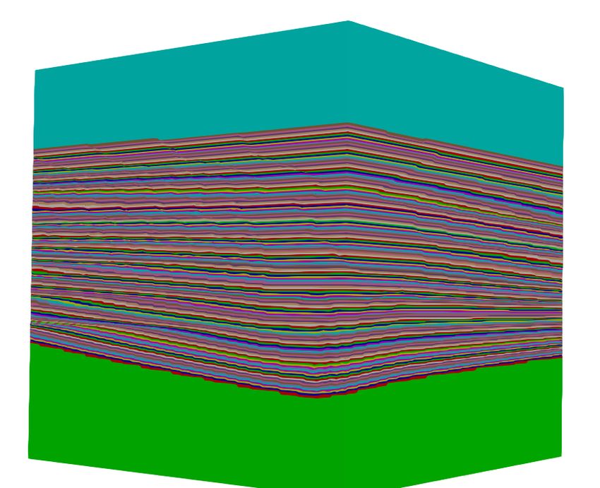
4.9.2 Photon creation - inverse transform sampling . . . . 29
4.9.3 Z-offset - look up table re-sampling . . . . . . . . . . 31
4.9.4 Propagation loop - removing branches . . . . . . . . . 31
4.9.5 Random number blocking . . . . . . . . . . . . . . . . 32
iv4.9.6 Manual caching in shared memory . . . . . . . . . . . 34
4.10 Discussion and future work . . . . . . . . . . . . . . . . . . . 35
5 A recipe for CUDA kernel optimization 39
6 Conclusion 43
v1 Introduction
This work explores the optimization of complex, highly divergent GPU
programs, using the IceCube projects photon propagation simulation (clsim)
as an example. All changes made to the code are documented and dis-
cussed. In addition, the methods used are generalized to other GPU codes
whenever possible.
The IceCube experiment operates a neutrino detector at the geographic
South pole [2]. Computer simulations are used to calibrate the sensor and
analyze observations by comparing them to the simulation results [5]. At
the time of writing, about 400 GPUs perform photon propagation around
the clock. It is still a major bottleneck in the physicists’ day to day work.
Some having to wait months for simulation results to be available.
The graphics processing unit (GPU) is used increasingly for general pur-
pose computation and computer simulation. All kinds of algorithms have
been successfully implemented on the massively parallel architecture [20].
It provides a higher computational throughput at lower energy consump-
tion compared to CPU architectures [10]. Many frameworks simplify pro-
gramming for GPUs. Achieving maximum performance on the other hand
is challenging. That is especially true for algorithms with a large discrep-
ancy of workload between threads. Programming models like CUDA and
OpenCL allow GPU code to be written on the thread level. The hardware,
however, executes instructions for 32 threads at a time. When a branch
needs to be executed for some of the threads, those that do not take the
branch are paused and can do nothing until the branch is completed. The
same happens when one of the threads stays in a loop longer than all the
others.
For specific cases, this problem can be solved in hardware. E.g. by
using RT-Cores, a special acceleration unit on current generation NVIDIA
GPUs, which accelerates the traversal of a geometrical acceleration struc-
ture. While this was mainly developed for ray tracing in a computer graph-
ics context, it has already been exploited for other applications [19]. Jachym
et al. use NVIDIA OptiX to simulate NC machining processes [15]. Wang
et al. make use of RT-Cores to simulate the interaction of tissue with ul-
trasound in real time [24], while Ulseth et al. simulate X-Ray Diffraction
Tomography [22]. Finally, Zellmann et al. use RT-Cores to draw force di-
rected graphs [25].
Another approach is to replace particularly complex parts of the calcu-
lation with an artificial neural network. It has been used for example by Guo
et al. to simplify a computational fluid dynamics solver [12], and more re-
cently by Hennigh et al. in NVIDIA SimNet an AI-accelerated framework
for physics simulation [14]. Evaluating a neural network on a GPU is a
well understood problem. Current generation NVIDIA GPUs even feature
1a second acceleration unit (the Tensor-Core), dedicated to evaluating neural
networks.
In other cases the individual algorithms need to be carefully analyzed
to find opportunities for optimization. Once parts of the code with perfor-
mance problems are identified, they can be modified or rewritten to better
fit the GPU. During the work on this thesis it was found, that the analysis of
the code can be far more complicated than the actual code changes applied
in the end. Finding out where and what to change is often the difficult part.
To successfully optimize the runtime of a program, the capabilities and
limitation of the programming language and target hardware need to be
understood as well as the analysis tools that come with it. In section 2.1
to 2.3 the CUDA programming model is introduced. It is then discussed
how it maps to the GPU hardware and what implications arise for perfor-
mance. RT-Cores, and using them with OptiX, as well as neural networks,
are discussed in section 2.4 and 2.5. In chapter 3, a number of analysis
methods are introduced. They will later be used to understand where
the majority of the time is spent during program execution and why it is
spent there. The process of optimizing the IceCube photon simulation code
(clsim) is explained in chapter 4. All changes made to the code and their ef-
fects are discussed in detail. In chapter 5 an attempt is made to generalize
the process of code analysis and optimization into a recipe to be applied to
other projects.
22 Background
In this section we give background information on a variety of topics. Those
need to be understood in order to follow later discussions.
2.1 Using the graphics processing unit for general computation
Once developed as a specialized hardware for 3D-rendering, the Graphics
Processing Unit (GPU) nowadays is a fully programmable processor de-
signed for parallel execution [10]. It features superior memory bandwidth
and computational throughput at similar power consumption compared
to a CPU design. I.e. less power is consumed when performing the same
calculation.
This is possible, because a GPU is meant to be used in a different way
than a CPU. The latter is designed to quickly execute a sequential thread of
a program, and depending on the model, can handle a few tens to these at
the same time. The GPU is designed for parallel execution first, executing
thousands of threads at the same time. It has much slower single-thread
performance in return. With different design goals, CPU and GPU use dif-
ferent amounts of transistors on specific parts of the processor. Figure 1
shows how on a GPU more transistors are used for processing, while less
are used for caching and flow control.
Figure 1: Example distribution of transistors for CPU and GPU. [10]
Inferior cache and flow control are compensated by hiding the latency
with more processing. GPU threads are light-weight, and it is cheap to
switch threads, while waiting for a memory access to complete. For this
to work properly, many more threads need to be provided than can be ex-
ecuted simultaneously. An application needs to expose a large amount of
parallelism, for it to be executed on a GPU efficiently.
In 2006 NVIDIA introduced CUDA. It allows programmers to directly
program GPUs for arbitrary tasks. Nowadays, many other frameworks to
3program GPUs exist. For example OpenCL, the directive based OpenACC,
as well as modern versions of graphics frameworks, like OpenGL, DirectX
and Vulkan. While CUDA does only work with NVIDIA GPUs, code can
be written in C++ and integrates well with the CPU part of the application.
It also comes without the cumbersome initialization code required to use
some of the graphics frameworks. In addition, many tools are available to
the CUDA programmer, like debugger [11], profiler [7], and an extensive
online documentation [10].
2.2 The CUDA programming model and hardware
When programming with CUDA, adding __global__ to a function defini-
tion marks the function as a kernel to be executed on the GPU. Inside the
kernel function, language extensions are available to make use of GPU-
specific functionality. When calling the kernel function, the desired num-
ber of GPU threads is specified. Similar to a parallel section in OpenMP, all
threads execute the same code. An index is used to differentiate threads.
This way, threads perform the same operations on different data.
Threads are partitioned into groups of program-defined size called thread
blocks. All threads of a block are executed by the same processor core or
Streaming Multiprocessor (SM). Threads of one block can synchronize and
access core-local memory (called shared memory). Programming an algo-
rithm that requires synchronization is simplified by the cooperative groups
API [13]. Blocks are further partitioned into warps of (on NVIDIA GPUs)
32 threads. Usually, threads of a warp are executed together, similar to
a SIMD vector processor. A single instruction controls the operation per-
formed on 32 pieces of data. Whenever threads of a warp take different
paths at a branch, all paths need to be executed for all threads. The threads
not taking a particular branch are simply marked as inactive. Additional
cooperation features are available for threads in a warp. That allows them
to, for example, directly access each other’s variables.
Programs that run on the GPU can access memory in multiple differ-
ent locations and on different hierarchical levels [10]. Figure 2 shows an
overview. The global memory is the GPU’s main memory, it can be read
and written from all GPU threads, as well as from the CPU. Access to global
memory is cached in L2 and L1 cache. The latter is local to every SM. Con-
stant memory can also be read by all threads. It is faster than global mem-
ory, as long as threads in a warp access the same memory location. Local
variables of the kernel function are stored in SM registers. When more vari-
ables are used than registers are available, data is stored in local memory
(register spilling). While local suggests it might be close to the processor
core, in fact it uses a section of the global memory. Lastly, there is shared
4Kernel
Global Local Texture Surface Shared Constant
Shared
L1 Cache
memory
PCIe Constant
L2 Cache
NVLINK Cache
GPU Global device memory
Figure 2: Overview of the GPU’s memory system. Parts marked in green exist in
every SM, parts in blue are global to the GPU.
memory. It is local to each SM and allows threads in a block to commu-
nicate. Hardware is shared with L1 cache. When more shared memory is
used, less L1 cache is available.
2.3 CUDA performance
As described in the previous chapter, CUDA makes it possible to write code
for the GPU similar to how one programs the CPU. Most hardware details
are hidden by the compiler and can be ignored for the purpose of writing
correct code. If performance is a concern however, the particularities of the
hardware need to be learned.
2.3.1 Memory
The compute power of GPUs improves with every generation, and Mem-
ory bandwidth can hardly keep up. Many applications slow down, because
instructions need to wait for a memory operation to complete. CUDA al-
lows individual threads to access different memory locations. In hardware,
however, memory access for all threads in a warp is combined to minimize
the number of transactions [10]. On newer GPUs (compute capability 6.0 or
higher) a memory transaction always loads 32 bytes, starting on an address
that is a multiple of 32 (i.e. 32 byte alignment). L2 cache uses lines of 128
byte length [23]. Older GPUs might use segments of 128 bytes even in L1.
As a result, not all access patterns can achieve the full bandwidth. In the
5simple, optimal case, a multiple of 128 bytes is requested in total, starting
at an address that is a multiple of 128. If the access is not aligned to an ad-
dress that is a multiple of 128 or 32, adjacent blocks need to be loaded, even
though the data is not used. In the worst case, every thread only accesses
very little data far apart. For example, threads access a single float with a
stride of 128 bytes. That would result in loading 4 kilobytes into L2 and 1
kilobyte from L2 to L1, however only 128 bytes contain data that is actually
used by the threads. It is therefore important to improve the access pattern
whenever possible. One way of doing this would be to load consecutive
data from global memory and store it in shared memory for later random
access. The CUDA best practice guide shows this technique as part of the
example Shared Memory in Matrix Multiplication (chapter 9.3.2.2) [9].
Data in constant memory is cached by the constant cache. It performs
best, when many threads access the same memory location. When different
constant memory locations are accessed from within one warp, the trans-
actions are serialized. If reading from many different locations is required,
global memory might be the better option [9].
When not enough registers are available on an SM to store all required
variables, some are stored in local memory instead. Since that is actually a
part of global memory, it is a lot slower to access those variables. If possible
one should minimize the amount of local variables, so that the use of local
memory is not necessary [9]. Shared memory can also be used to store data
that does not fit into registers, especially if it is relevant to different threads.
2.3.2 Occupancy
To sufficiently hide the latency of memory access, synchronization and im-
balance, it is important that each SM always has something ready to com-
pute. Exposing enough parallelism in an algorithm, so that many more
threads than processors are available, is only the first step. The amount of
registers and shared memory per SM are limited. If a kernel uses a high
amount of those resources, it will limit the number of blocks that can reside
on the same SM [10]. Setting an appropriate block size is also important.
Since warps contain 32 threads (on NVIDIA GPUs), block sizes should be
a multiple of 32. Values between 128 and 256 are a good starting point [9].
The optimal value does however, depend on the kernel in question and the
type of GPU used. It is best found by experimentation. Multiple smaller
blocks on one SM are often better at hiding latencies than a single large
block.
62.3.3 Computation and control flow
Sometimes performance of a kernel is not limited by memory, but compu-
tation. In that case, the mathematical precision needed to solve the problem
should be considered carefully. Most GPUs work much faster with floating
point numbers of single precision (32 bit), than double precision (64 bit).
The compiler flag -use_fast_math can be used to replace all calls to math
library functions (sqrt(), pow(), exp(), etc.) with the less precise, but
faster intrinsic functions (__sqrt(), __pow(), __exp()) [9].
Because warps of 32 threads are executed together, control flow in-
struction – where threads of a warp take different branches – should be
avoided whenever possible. Sometimes, work can be reordered so that
threads of the same warp take the same branch. The CUDA best practice
guide gives the example of having a branching condition that depends on
(threadIdx / WARPSIZE), instead of one that depends on thread index di-
rectly [9]. When branching can not be avoided, the branch itself should be
made as short as possible.
2.4 NVIDIA Optix
OptiX is NVIDIA’s framework for GPU based ray tracing [21]. It provides
a programming model similar to the Vulkan and DirectX raytracing mod-
ules. The programmer provides different CUDA functions for ray gener-
ation and reacting to hit and miss scenarios [8]. OptiX itself handles the
build and traversal of a geometrical acceleration structure to narrow down
the number of primitives that need to be tested for intersection. It fea-
tures build in ray intersection tests for standard geometry like triangles
and curves. The user can also provide his own CUDA function to test for
intersection with arbitrary geometry.
On newer GPUs, OptiX makes use of the RT-Cores, a special unit on
the GPU to accelerate ray tracing. RT-Cores perform the traversion of the
geometrical acceleration structure, as well as ray-triangle intersections, in
hardware. That allowed the RTX2080 GPU to perform raytracing about 10
times faster than the GTX1080 [16].
Version 7 of the OptiX framework closely integrates with CUDA. Port-
ing a CUDA application to OptiX is therefore relatively straight forward [8].
2.5 Artificial neural networks on GPUs
The building block of an artificial neural network (ANN) is the neuron. It
has several inputs, each with a corresponding weight, a bias value, and an
output. The value of the output is computed by multiplying every input
value with its weight, adding them up, together with the bias, and applying
a nonlinear function to the result (called activation function). Combining
7many of those neurons in a network results in a nonlinear function that
turns input values into output values depending on the weights and biases
of all neurons in the network.
In this context, learning or training the network, is the process of set-
ting the weights and biases to specific values, so that the network exhibits
the desired behavior. This can be achieved by evaluating the network for
an input with a known desired output value. The result of the network’s
calculation is compared to the desired output and and the error is calcu-
lated. Weights and biases are then changed to minimize the error. For the
network to generalize well to new data, many such training iterations with
lots of different example data need to be performed. Over time, more so-
phisticated methods for building and training neural networks for specific
applications have been developed. [17]
GPUs are well suited to perform the many evaluations needed for train-
ing and using an ANN in parallel. In addition, the evaluation can be
mathematically described as a series of matrix multiplications. The Tensor-
Cores on NVIDIA’s GPUs are hardware units to accelerate matrix multipli-
cation. They have been specifically designed to speed up the evaluation of
ANNs [16].
83 Methods of code analysis
When optimizing a program’s execution time, it is essential to know what
is taking up time and to understand why. Only that allows to decide about
code changes in an educated way. It is also helpful to estimate how much
improvement can be expected from a specific change, and how good the
current implementation is considering the processor’s capabilities. While
wall-clock time of different functions can be easily measured and compared
in a single threaded application, analyzing GPU code is more difficult.
In this section the tools and methods used to analyze and understand
the program in detail will be presented.
3.1 Wall-clock time
The simplest way to measure the runtime of a program part on the CPU
is to use the time measurement features native to the chosen programming
language. Multiple measurements should be taken and averaged, since
other processes running on the system will influence the runtime. There-
fore it needs to be ensured that the measured function does not have any
side effects that would multiple runs. Measuring time like this is only pos-
sible in a single threaded context on the CPU. It can still be used in GPU
computing to measure the duration of an entire kernel launch. This is es-
pecially useful when comparing to older versions of the same code or dif-
ferent implementation methods (OpenCL vs. CUDA, CPU vs. GPU).
Listing 1 provides an example of measuring wall-clock time of a CUDA-
kernel in C++. We call cudaDeviceSyncronize() to make sure the GPU fin-
ishes executing the kernel before the timer is stopped.
Listing 1: Measuring wall-clock time of CUDA Kernel in C++
1 #include
2
3 void wctKernel(int numRuns)
4 {
5 runMyKernel();
6 cudaDeviceSyncronize();
7
8 auto start = std::chrono::steady_clock::now();
9 for(int i=0; i3.2 Nsight Compute
Nsight Compute is the profiling software provided by NVIDIA to perform
an in-depth analysis of CUDA code while running on a GPU. A CUDA ap-
plication can be launched interactively from within Nsight or by using the
command-line tool. Collected data can then be viewed in the user interface
and compared to previous profiles.
The information collected by Nsight includes (but is not limited to) a
detailed analysis of memory usage – with cache usage – and information
on how many threads are inactive due to warp divergence. It also shows
how often the execution of a thread has to be suspended because the pre-
requisites of a given instruction are not met (stall). Most metrics can be
correlated with PTX/SASS instructions as well as lines of C++ code1 . In ad-
dition more general information about the kernel launch is available. The
Occupancy, shared memory and register usage is calculated and a speed of
light analysis as well as a roofline plot are generated (see the next two sec-
tions).
The full documentation of Nsight, as well as a guide on kernel profiling
are available on the NVIDIA website [7] [6].
3.3 Speed-Of-Light analysis
Nsight Compute includes a section on speed of light analysis. It gives a high
level overview on how effectively the program uses resources available on
the GPU. The achieved utilization of the GPUs streaming multiprocessors
(SM) is given as a percentage of the theoretical maximum for the used GPU.
Similarly, the used memory bandwidth is displayed as a percentage of the
theoretical maximum memory bandwidth.
Together those two numbers are a useful indicator for the current state
of the code. A high value in SM usage indicates that the code makes good
use of the computing power and can be sped up by simplifying the cal-
culations or transferring work to the memory system (e.g. precomputing
/ reusing values). A high value in the memory usage indicates that the
code saturates the memory system and can be sped up by improving the
memory access pattern, cache usage or reducing the number of memory
accesses. If both values are low, the cause might be synchronization and
waiting, warp divergence, low occupancy or similar. It can also happen
when a bad memory access pattern is used and only a few computations
are executed on the data. In case that both values are high, the program
already uses the GPU efficiently and a major change of the algorithm will
be required for further speed-up.
1
Code needs to be compiled with the option –lineinfo to display source code in Nsight
Compute
10If a profiling tool like Nsight Compute is not available, the number of
memory access and floating point operations could also be counted by
hand and compared to the device’s capabilities.
Figure 3: Example speed of light analysis performed in Nsight Compute.
3.4 Roofline plot
To better visualize how the program in question uses compute and mem-
ory resources, a roofline plot can be used. An example is given in figure 4.
The X-Axis shows arithmetic intensity, i.e. the number of floating point op-
erations per byte of memory access. The Y-Axis shows overall performance
in floating point operations per second. The theoretical peak performance
and peak memory bandwidth are plotted in the diagram, resulting in a
horizontal and diagonal line respectively. Together they form the roofline
which shows the maximum performance that can be achieved for a given
arithmetic intensity. The arithmetic intensity of the program in question is
then calculated and also plotted in the diagram [6].
With this kind of diagram, the impact of changing the arithmetic inten-
sity is easily estimated. One can also make predictions of how the code
would perform when moved to other hardware, or changed between 32
and 64 bit floating point numbers. More information about the roofline
model and its uses can be found on the NVIDIA developers blog [18].
Figure 4: Example roofline created with Nsight Compute. The diagonal line shows
arithmetic intensities limited by bandwidth. The upper horizontal line is
32bit floating point performance, the lower horizontal line is 64bit float-
ing point performance.
113.5 Measuring individual parts of the code
When a complex algorithm is implemented inside one single CUDA-kernel,
it is difficult to identify which part of the code has potential for optimiza-
tion. To analyze the individual parts of the algorithm, the code must be
modified. It can be split up into multiple kernels, which are then analyzed
individually. Alternatively parts of the algorithm can be temporarily re-
moved.
One must be aware that doing so can change the behavior of the re-
maining code in unexpected ways. The compiler optimization might re-
move code if the result is unused or a certain condition is always true or
false. Tools like godbolt 2 can be used to inspect the generated assembly and
verify the measurement works as intended.
Even if the code remains intact, removing one part of the code can
change the behavior of the other parts. E.g. in the removed part of the
code a variable is set to a random value and the measured part of the code
contains a branch based on that value. Results obtained by this method
must be considered carefully and should only be seen as estimates.
3.6 Counting clock cycles
In CUDA device code, the function long long int clock64(); can be used
to read the value of a per multiprocessor counter, that is incremented with
every clock cycle. Taking the difference of a measurement at the beginning
and end of a section of device code in every thread will yield the number
of clock cycles it took to execute that part of the code.
However, in general, not all those clock cycles have been spent on in-
structions from that particular thread. A threads execution might be paused
by the scheduler to execute instructions from another thread in-between.
The method can still be useful for approximate comparisons.
3.7 Custom metrics
Measuring custom metrics can improve the understanding of the code and
its reaction to different input data. E.g. a loop with an iteration number
computed at runtime looks expensive at first glance. Measuring the actual
number of loop iterations might reveal, however, that in 99% of the cases
only one iteration is performed.
On the GPU, metrics can be measured per thread, or per block. They
are downloaded to CPU memory and combined for analysis. E.g. in form
of an average or histogram.
2
godbolt compiler explorer: https://godbolt.org/
123.8 Impact estimation
When a performance problem and its cause have been identified, fixing it
in a way that maintains the correctness of the code can be hard and time
consuming. It is helpful to estimate the impact of that particular problem
on the overall runtime first.
To do that, the problem’s cause is eliminated in the simplest way possi-
ble, even if that means incorrect results are produced. Then the analysis is
repeated, to verify that the cause was identified correctly and the problem
does not occur anymore. The new time measurement shows how big the
impact of that particular problem is on the overall performance. Now an
informed decision can be made on whether or not it is worth to work on
mitigating the problem in a way that does produce the correct results.
3.9 Minimal working example
To estimate the performance impact of a certain optimization, the simplest
possible version of the new method can be implemented in a standalone
application. Inputs and outputs for the specific function call are saved to
a file in the original application. They are then loaded in the minimal ex-
ample application. Performance and correctness of the new method can be
tested before any potentially time consuming integration work is done.
When testing for correctness, it can also be useful to implement the sec-
tion in question using a high level programming language on the CPU.
This only works, as long as no GPU specific operations are involved. E.g.
when changing a function of a physical model that is called by every GPU
thread individually. The usage of a high level language allows for sim-
ple comparison of the output of both functions, by using built-in statistical
tools and plotting facilities. It also simplifies debugging and makes it easier
to feed the function with specific input data, such as randomly generated
test-cases.
3.10 Incremental rewrite
Sometimes a kernel is too complex to be understood and analyzed as a
whole in the detail needed for optimization. Performing an incremen-
tal rewrite can help to reveal opportunities previously hidden under that
complexity. Many of the aforementioned techniques are applied iteratively.
Therefore, it can be quite time consuming.
When performing an incremental rewrite one starts from a new, empty
kernel. Functionality is added incrementally until all features of the origi-
nal code are restored. In every step the program is profiled and compared
to the previous version. Whenever it moves further away from the roofline
or the speed of light, or when the wall-clock time increases considerably,
13the newly added code is considered for optimization. The techniques de-
scribed in this chapter are then applied to analyze the newly added code.
If applicable, the minimal working example technique is used to derive and
test an alternative implementation of the feature in question.
One problem with this technique is, that a regression test – to compare
against the original code for correctness – can only be performed after the
incremental rewrite is completed. Usually, many modifications have been
made by that point, which makes debugging difficult. When performing
especially big changes to a single part of the program, it is preferred to in-
tegrate them into the original code to check for correctness, before moving
on to the next step. While this makes the technique even more time con-
suming, it is preferred over having a broken program in the end, without
any way to isolate the bug. It prevents the programmer from losing sight
of the bigger picture and getting lost in details.
The incremental rewrite technique is a last resort, to be used after opti-
mizations on a broader scale do not yield further progress. See section 4.9
for an example of how the technique is applied to the IceCube simulation
code.
144 Analysis and optimization of the IceCube simula-
tion
In this chapter, the process by which the IceCube photon propagation sim-
ulation code (clsim) has been optimized, is described in detail. Methods
presented in the previous section are used, to identify parts of the code
with optimization potential. In every subsection a different optimization
attempt is discussed.
It can be read to familiarize oneself with the current state of the IceCube
clsim code. Alternatively, it can be seen as an example on how the different
techniques from section 3 are used together when optimizing an actual pro-
gram. In addition, cases in which a particular optimization can be applied
to other programs are highlighted.
4.1 The IceCube experiment
The IceCube Neutrino observatory operates an array of sensors embedded
into one cubic kilometer of ice at the geographical South pole [2]. In total
5160 optical sensors are buried in the ice. They are ordered in a hexagonal
grid between 1450 and 2450 meters below the surface.
Neutrinos that interact with the ice produce secondary particles. Those
move faster then the speed of light in the medium, which causes them to
generate photons by the Cherenkov Effect [4]. The photons are then detected
by the IceCube sensors. Properties of the neutrino can be calculated from
the detected photons [1]. That allows scientists to derive information about
the origins of the neutrinos. Those can be cosmic events like exploding
stars, gamma-ray bursts and phenomena involving black holes and neu-
tron stars.
Figure 5: Images of a 3D model, showing the IceCube detectors and ice layer
model. Created by Ramona Hohl.
15To operate the experiment and analyze the data a multitude of com-
puter programs are used. This work is focused on the simulation of photon
behavior in the ice. It is needed to find potential sources of systematic er-
rors, calibrate sensors and reproduce experiment results for analysis [5].
4.2 The IceCube photon propagation simulation
A Monte-Carlo method is
employed to simulate the
has thread valid
photon’s movement through photon
the different layers of ice
no
(each of which has individ-
ual optical properties). In- create new photon
put to the simulation are so from step
yes
called steps. They represent
sections of the neutrino’s determine distance
path where photons with to absorbtion
approximately constant prop-
erties are generated. Af- determine distance
ter loading those steps into to next scatter
GPU-memory one thread
is launched for every step. propagate until
Steps are handled com- scatter or absorbtion
pletely independent from
each other. For every step
check collision
photons are generated us-
ing a random distribution. yes no
They are then propagated
through the ice for multiple record hit and check for absorbtion
iterations [5]. invalidate photon
yes
no
invalidate photon
scatter
Figure 6: Overview of the photon propagation al-
gorithm (explanation on the next page).
16Each iteration consists of four parts:
• First the photon is moved on a linear path through a number of ice
layers, until it reaches the next scattering point or is absorbed. A
random number from an exponential distribution represents the dis-
tance to the scattering point. It is weighted by the scattering proper-
ties (scattering length) of the ice. Different layers have different scatter-
ing lengths. The algorithm iterates over the layers. Distance traveled
through a layer is weighted by the layer’s scattering lengths and then
subtracted from the randomly picked distance. The iteration stops,
when the distance to the next scattering point becomes zero. It also
stops if the photon is absorbed by the ice. When that happens also
depends on the properties of individual ice layers [3].
• Next, collision detection is performed. The algorithm checks whether
or not the linear path between the previous and next scattering point
intersects with any of the spherical sensors. A spatial data structure,
similar to a uniform grid, but modified based on the actual distri-
bution of sensors in the ice, is used to narrow down the amount of
spheres that need to be tested directly.
• If a photon does hit a sensor, it is stored as a hit in the results buffer.
If it gets absorbed, it is simply discarded. Otherwise the photon is
scattered. A new direction is chosen based on a random number. The
Henyey-Greenstein and simplified Liu scattering functions are com-
bined to match the actual ice behavior [3].
• Finally, photon variables – like position and direction vectors – are
updated. If the thread does not have a valid photon anymore (it hit a
sensor or was absorbed) a new photon is created from the step. This is
repeated until all photons specified in the step have been simulated.
The clsim simulation was originally implemented with OpenCl and ported
to CUDA by Ramona Hohl at NVIDIA.
4.3 Initial setup
Starting work on the IceCube code, Ramona Hohl set up facilities to mea-
sure wall-clock time (section 3.1) and the IceCube scientists provided us
with a performance benchmark and regression test. This allows us to com-
pare the future changes with the original code. Ramona Hohl then ported
the OpenCL code to CUDA. We picked the NVIDIA RTX 6000 GPU as our
working hardware, but also checked the performance on other GPUs from
time to time.
The original code made use of the fast math compiler optimization and
it is still used for the CUDA compiler. The simulation already uses single
17precision (32 bit) floating point numbers. It was decided by the scientists
that reducing precision even more could result in problems at the edges of
the simulated domain.
Focusing the optimization on a single code path and removing all #ifdef
sections that belonged to unrelated settings proved helpful in the long run.
It makes the code easier to understand and helps to focus ones attention on
the important parts.
The use of CUDA over OpenCL alone sped up the code by a factor
of 1.18x.
4.4 Occupancy and constant memory usage
Profiles taken with Nsight Compute indicate a medium occupancy and prob-
lems with the way the kernel accesses memory. Only 0.57% of the devices
memory bandwidth seems to be utilized even though we know that data is
constantly accessed from various look up tables that store physical quan-
tities. It turns out that this data is stored in constant memory and Nsight
does not include constant memory in its statistics. Information on con-
stant memory usage is (at the time of writing) only available in the raw data
view under idc_request_cycles_active. We filed a feature request with
the Nsight team to include that functionality in future releases.
To increase the occupancy, Ramona Hohl set the size of a thread block to
512 and limits register usage, so four thread blocks reside on one SM. The
__launch_bounds__(NTHREADS_PER_BLOCK, NBLOCKS_PER_SM) attribute, used
in the kernel declaration, allows to make these settings. Those properties
are also exposed to the user as compile time settings, as different values
might be needed depending on the GPU used. It is recommended to test
block sizes of 128, 256 and 512 threads, while using as many blocks per SM
as possible without spilling registers (limiting the available registers per
thread so much, that thread variables need to be stored in local memory
instead of registers). The increased occupancy leads to an additional 1.09x
speedup.
Photons simulated by threads of the same warp or thread block, might
take vastly different paths through the ice. Therefore ice properties and
geometry data are read from memory at random addresses without any
particular order or system. It also introduces warp divergence at branches.
Ice and geometry data are stored in constant memory in the original ver-
sion. Reading from constant memory is faster than normal global memory,
when only a few different memory locations are accessed by the threads of
a warp.
Using global memory for all randomly accessed data results in an ad-
ditional 1.48x speedup. That makes an overall improvement of 1, 91x for
now.
184.5 Detailed analysis
The Nsight Compute profile now shows a SM utilization of 66% and a mem-
ory utilization of 31.5%. While the arithmetic intensity of the code is high
enough to not be bound by memory, it does not quite reach the roofline.
One possible reason is the high warp divergence (on average, only 13.73
out of the 32 threads per warp are doing work).
While using global memory is faster than constant memory when ac-
cessing randomly, that is still not the preferred access pattern. Overall
memory bandwidth does not seem to be a problem, however, specific sec-
tions of the code might still be slowed down while waiting for an inefficient
memory access to complete.
A better understanding of which parts of the code use up most of the
time is necessary. Therefore, further timings with a modified kernel code
were run (see section 3.5). Ramona Hohl also used CUDA’s clock cycle
counting mechanism (section 3.6) to make similar measurements. Figure 7
shows the percentage of the total runtime different parts of the code take
up according to all the used methods of measurement. While the absolute
results vary from method to method a trend can be identified. Collision
testing with the sensors takes up about one third of the runtime, same as
propagation through the different ice layers. The last third is made up of
scattering and path update, as well as photon creation and initialization
code.
Figure 7: Different parts of the clsim kernel measured using 3 different methods.
The kernel was modified in 1 by removing the part to be measured, and
in 2 by removing everything but the part to be measured. Method 1 does
not allow the measurement of photon creation and method 2 overesti-
mates it, as miscellaneous setup work is included in the measurement.
19Upon collision with a sensor, data about that collision is stored in a
buffer in global memory and later transferred to the CPU. All threads on
the device might write to this global buffer. To keep track of where the next
element needs to be written, a counter variable is incremented atomically.
Since storing is conditional (only if a sensor is hit), all other threads of the
warp need to wait while the branch is executed. Luckily, only about 0.029%
of photons ever collide with a sensor. The others are absorbed by the ice
early, or scattered in the wrong direction. Dividing by 26 – the number of
collision checks that happen for a photon on average (see next paragraph) –
yields only a 0.001% chance that a photon is stored after one particular colli-
sion test. The overhead for the atomic operation and the branch is therefore
very small. An attempt to collect collision events in shared memory first,
and move them to global memory later, did not result in much improve-
ment. It was decided to use the shared memory for other optimizations
later on.
Photon paths are based on a random number generator, so some are
longer than others. To better understand the imbalance in workload intro-
duced by this, Ramona Hohl measured the number of propagation loop
iterations it takes for one photon to be simulated (equivalent to the num-
ber of scattering events). The results can be seen in figure 8. The average
number of iterations is 25.9, which also explains while photon creation only
has a minor impact on performance. For every photon created, propaga-
tion, scattering and collision testing are performed about 26 times. While
the range of iterations per photon varies considerably, having many pho-
tons per thread reduces the imbalance between threads. In the benchmark,
which uses 200 photons per thread, values range from 19 to 35 (see figure 9).
20Figure 8: Histogram shows how many photons take a given number of propaga-
tions before colliding or being absorbed. The Histogram is cut at 200
propagations, however, the maximum amount is 622.
Figure 9: Histogram hows how many steps have a given average number of prop-
agations per photon.
During production usage, different threads do not usually have the
same number of photons to process. Only photons with similar physical
properties are grouped together and processed by one thread. A second
benchmark was created – which is referred to as shuffled from here on – to
21reflect this behavior. The additional imbalance introduced by the shuffled
initial conditions slows the code down by a factor of 1.3.
As mentioned above, the Nsight profile shows a considerable amount
of warp divergence. Only 13.7 threads per warp are active on average.
For testing, the random number generator seed was set to the same value
for every thread in a warp. In addition, those threads were modified to
work on the same step. That artificially eliminates all divergence and the
overall computing work stays the same. Now 30.8 threads per warp are
active on average and the code is sped up by 3x. In this modified code,
threads of a warp simulate the exact same photon and path, which does not
yield useful physical results. It will be impossible to eliminate divergence
completely in the IceCube code. Nevertheless, this experiment shows the
big performance impact of warp divergence.
4.6 Per warp job-queue, a pattern for load balancing
To balance the workload among the GPU threads – and prevent resulting
warp divergence – what we call a per warp job-queue was implemented. The
pattern can be applied whenever work items of different length are packed
into bundles of different size for processing on the GPU.
4.6.1 The problem: imbalance
In the IceCube simulation code a photon can be considered a work item.
Multiple photons with similar properties are bundled together in what is
called a step. One GPU thread is tasked with the propagation of all pho-
tons from one step. Steps can contain different amounts of photons, whose
propagation will take different amounts of iterations. That introduces im-
balance, which in turn leads to warp divergence. Some threads will finish
their work faster than others. The GPU has a built-in scheduler, which dy-
namically assigns new thread blocks to the SMs once it becomes available.
However, code is executed in warps of 32 threads. Up to 31 of those could
be idle, waiting for the last thread to finish its step (if it contains more pho-
tons than the steps of neighboring threads).
4.6.2 Implementation
Instead of using one thread to handle each bundle, an entire warp is used.
The work items from the bundle are shared among all 32 threads. Shared
memory and the CUDA cooperative groups API make for fast communica-
tion between the threads. When a thread finishes executing one item, it
will take the next from a queue in shared memory. Whenever the queue
is empty, the 32 threads come together to fill it with new work items from
22the bundle. We provide an example implementation – without IceCube
specific functionality – in listing 2 and 3 .
Listing 2: Per warp job-queue
1 #include
2 namespace cg = cooperative_groups;
3
4 void perWarpJobQueue(cg::thread_block_tile& group,
5 Bundle& bundle, Item* sharedItemQueue,
6 int& numItemsInQueue)
7 {
8 int itemsLeftInBundle = bundle.getNumItems();
9 int currentItemId = -1;
10 Item currentItem;
11 group.sync();
12
13 // load/create items for direct processing
14 if(group.thread_rank() < itemsLeftInBundle) {
15 Item = bundle.getItem();
16 currentItemId = 0; // set any valid id
17 }
18 itemsLeftInBundle -= group.size();
19
20 fillQueue(...);
21 group.sync();
22
23 // loop as long as this thread has a valid item
24 while(currentItemId>=0) {
25 doSomeWorkOn(currentItem);
26 if(workDone(currentItem))
27 currentItemId = -1;
28
29 if(numItemsInQueue>0 || itemsLeftInBundle>0) {
30 if(currentItemIdin shared memory and also need to be unique for every warp. The mem-
ory pointed to by Item* sharedItemQueue needs to be big enough to store
32 items.
The variable currentItemId is >= 0 when the current thread contains
a valid item. If the item was loaded from the queue, it denotes the place
in the queue that particular item was loaded from. It is not usable in the
case that bundle::getItem(); requires a unique ID for each item. However
a unique id for item creation could be calculated as itemsLeftInBundle -
group.thread_rank().
Interesting to note is, that group.sync() is called inside a loop and a
branch repeatedly. This would be considered unsafe in the general case.
Here however, it is guaranteed that either all threads or no threads will
execute the sync command. The condition in line 29 asks, if any items are
left in the queue, or the bundle. This is the same for all threads. In addition,
no thread can ever leave the main processing loop (line 24) as long as that
condition evaluates to true.
Listing 3: Filling and accessing the queue
1
2 // fills the queue with new items
3 void fillQueue(cg::thread_block_tile& group,
4 Bundle& bundle, int& itemsLeftInBundle,
5 Item* sharedItemQueue, int& numItemsInQueue)
6 {
7 if(group.thread_rank() < itemsLeftInBundle)
8 sharedItemQueue[group.thread_rank()] = bundle.getItem();
9 if(group.thread_rank() == 0) {
10 int d = min(group.size(),itemsLeftInBundle);
11 numItemsInQueue = d;
12 itemsLeftInBundle -= d;
13 }
14 itemsLeftInBundle = group.shfl(itemsLeftInBundle,0);
15 }
16
17 // grabs an item from the queue
18 void grabItemFromQueue(Item* sharedItemQueue, int&
numItemsInQueue, Item& currentItem, int& currentItemId)
19 {
20 // try to grab a new item from shared memory
21 currentItemId = atomicAdd(&numItemsInQueue,-1)-1;
22 if(currentItemId >= 0)
23 currentItem = sharedItemQueue[currentItemId];
24 }
If the processing of an item is not iterative and all items take approxi-
mately the same time, the pattern can be simplified accordingly. The same
applies if creating a work item from the bundle in place is faster than load-
ing it from shared memory. In this case the queue stored in shared memory
would not be needed.
244.6.3 Results
Unfortunately, the pattern shown above has a non neglectable overhead
over the naive implementation. It also uses additional local variables. In
the clsim code, some data is stored in a local variable at photon creation,
just to be written to the output buffer in the unlikely case that a photon
does actually hit a sensor. According to the original author of the program,
that data was mostly used for debugging purposes and is no longer needed
as part of the programs output. Removing these local variables allows most
of the job-queue variables to be stored in registers and reduces the amount
of local memory accesses.
In the default benchmark, the big number of photons in each step aver-
ages out the difference in loop iterations between threads. Here, the version
of the code using the job-queue pattern performs similarly to the original
code. When running the shuffled benchmark however – where every step
has a different number of photons – the job-queue is about 1.26x faster than
the naive implementation.
As the queue holds 32 elements at a time, one would expect that round-
ing the number of work items (photons) in each bundle (step) to a multiple
of 32 might improve the performance. However, that is not necessarily the
case in practice. It might make a difference in a program, where loading or
generating a work item from the bundle is more time consuming, or when
the amount of items per bundle is low.
What does improve the performance of the code in any version how-
ever (with and without load balancing), is using bundles that contain more
work items (see figure 10). In the case of the IceCube simulation, photons
in one step are assumed to have similar physical properties. Reducing the
number of steps would therefore mean to decrease the resolution of the sim-
ulation, even when the overall photon count is kept constant. The user has
to decide how many different steps the photons need to be partitioned in,
to reach the desired balance between accuracy and speed.
25Figure 10: Increasing the size of the steps at constant photon count improves per-
formance. Runtime is given in nanoseconds per simulated photon.
4.7 NVIDIA OptiX for collision detection
At this point about one third of the runtime is spent performing collision
detection between the photons and sensors. The path, on which a photon
travels between two scattering events, is assumed to be linear. It has an
origin, a direction and a length. The collision detection needs to find out
whether or not this path intersects with one of the 5160 spherical sensors.
To prevent testing every photon path with every sensor, the code uses a
spatial datastructure. It is similar to a uniform grid, but modified based on
the specific layout of the sensors. As the problem seems to be very similar
to the intersection tests performed during ray tracing, we decided to use
the dedicated RT-Cores present on current generation NVIDIA GPUs.
The RT-Cores can not be utilized directly from CUDA though. Instead
the code needs to be ported to the Optix raytracing framework (using the
vulkan or DirectX graphics API is also possible in theory). The current ver-
sion of Optix shares many concepts with CUDA, porting the code is there-
fore not too difficult.
We started by exporting some of the photon paths from the CUDA ap-
plication and imported them into a new Optix program. That sped up the
pure collision detection part of the code by roughly 2x. After including the
rest of the simulation into the OptiX program, it ran 1.39 times slower than
the CUDA version. One possible explanation would be, that the OptiX tool-
chain does not optimize as aggressively as the CUDA compiler. In addition
some of the tuning parameters, as well as access to shared memory, are not
26You can also read