Popularity Growth Patterns of YouTube Videos: A Category-based Study
←
→
Page content transcription
If your browser does not render page correctly, please read the page content below
Popularity Growth Patterns of YouTube Videos:
                                A Category-based Study

                                Shaiful Alam Chowdhury and Dwight Makaroff
            Department of Computer Science, University of Saskatchewan, Saskatoon, SK, S7N 5C9, CANADA
                                         {sbc882, makaroff}@cs.usask.ca

Keywords:      Workload characterization: multimedia applications: content distribution; time-series clustering

Abstract:      Understanding the growth pattern of content popularity has become a subject of immense interest to Internet
               service providers, content makers and on-line advertisers. This understanding is important for the sustainable
               deployment of content distribution systems. A significant amount of research has been done in analyzing the
               popularity growth patterns of YouTube videos. Unfortunately, little work has been done that investigates the
               popularity patterns of YouTube videos based on video object category. In this paper, we perform an in-depth
               analysis of the popularity pattern of YouTube videos, considering video categories. We find that the time
               varying popularity of different YouTube categories are different from each other. For some categories, views
               at early ages can be used to predict future popularity, whereas for some other categories, predicting future
               popularity is a challenging task and requires more sophisticated techniques (e.g. time-series clustering). The
               outcomes of these analyses can be instrumental towards designing a reliable workload generator, which can be
               further used to evaluate different caching policies and distribution mechanism for YouTube and similar sites.

1    INTRODUCTION                                                types of systems. The methodology we have devel-
                                                                 oped is useful for UGC sites that have a single cache
YouTube and other user generated content (UGC)                   for the region of requests captured.
sites have altered the way people watch video on the                 In this paper, the time-varying global viewing pat-
Internet. YouTube was the 4th most accessed Inter-               terns of a sample of YouTube videos from their up-
net site in 2007 (Cheng et al., 2007), and its use was           load time are analyzed, considering video category.1
increasing over time in a power-law manner. Re-                  We present the results of one data collection period
cent studies continue to support two central observa-            (5 months of views of videos uploaded in 2 consecu-
tions: 1) increasing number of videos and users (Ding            tive days); a previous dataset showed similar charac-
et al., 2011; Siersdorfer et al., 2010) and 2) dissatisfy-       teristics and is not evaluated here. Our results show
ing experiences of users in watching YouTube videos              that different categories exhibit different viewing pat-
(Khemmarat et al., 2011). Other recent studies (Gem-             terns in terms of overall popularity and detailed pop-
ber et al., 2011; Labovitz et al., 2010; Maier et al.,           ularity over time. We confirmed that the number of
2010) suggest that YouTube is the most bandwidth in-             views of the popular videos follows a Zipf distribu-
tensive service of today’s Internet, and it accounts for         tion for most categories, whereas views of the unpop-
20-35% of Internet traffic.                                      ular videos follow a heavy tail distribution. We also
    Much research has been done investigating re-                show that time-series clustering can be successfully
quest characteristics from both client (Gill et al.,             used to understand the growth patterns for the cate-
2007; Zink et al., 2009) and server perspectives                 gories where early popularity cannot be used to pre-
(Borghol et al., 2011; Cha et al., 2009; Ding et al.,            dict future popularity of a video.
2011; Figueiredo et al., 2011) in order to enable im-                These observations contribute to a better under-
proved service. However, none of this earlier work               standing of the popularity dynamics of YouTube
considered the types of video objects. This aggregate            videos, enabling realistic testing scenarios for devel-
data may not tell the whole story.                               oping and evaluating various design parameters for
    A proper understanding of YouTube’s workload                 UGC sites. While the request patterns for different
will aid in the design of new systems, as well as ca-
pacity planning, and network management for similar                 1 as   defined by the uploader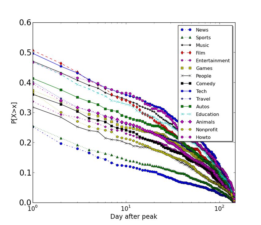
categories may vary around the world, our dataset and     posed. For instance, it is claimed that video requests
analysis provide a case study that shows that cate-       in YouTube follow a Zipf distribution (Gill et al.,
gory differences persist in global access patterns, and   2007), which is different from other works that con-
therefore will exist in each region. Our analysis en-     sider global request patterns. For our purposes, global
ables the development of category-specific workload       access patterns are essential.
generators which can be combined to form the input            2.5 million YouTube videos were obtained using
for simulators and prototype systems. While devel-        related video links (Cheng et al., 2007). Access pat-
oping and evaluating a comprehensive workload gen-        terns of the popular videos did follow a Zipf-like dis-
erator remains as future work, we have a strategy for     tribution, in spite of having a heavy-tailed section
generating synthetic requests on a category basis and     in the distribution curve. Data collected indicated
present preliminary results which match reasonably        that the YouTube network is similar to small world
well for two categories: News and Music.                  networks, and P2P techniques could be successfully
    The remainder of the paper is organized as fol-       applied, contradicting earlier findings (Zink et al.,
lows. Related work is described in Section 2. Section     2009). Their dataset is likely to be biased to popular
3 explains the data collection methods of our study.      videos because of the crawling approach, and popu-
We discuss the characterization of the request patterns   larity over time is not investigated in detail.
in Section 4, and use the information from views over         A recent approach to investigate growth patterns
time to develop a workload generator for two cate-        in YouTube video requests was to use Google charts
gories in Section 5. Section 6 provides conclusions       to collect views over time (Figueiredo et al., 2011).
and future work.                                          They analyzed the time-varying viewing patterns of
                                                          popular videos, deleted videos and randomly selected
                                                          videos. Popular videos usually experience a huge
                                                          number of views on a single peak day or week. Unfor-
2    RELATED WORK                                         tunately, using the Google charts API is not sufficient
                                                          to have a proper, fine-grained understanding of the dy-
Previous request characterization and video popular-      namics of video popularity as Google charts API al-
ity analysis has been used to investigate the feasibil-   ways returns 100 data points, regardless of video age.
ity of different content delivery streaming techniques,       Recent work was done on nearly 30,000 videos,
and to design and evaluate caching policies/systems       collected by using the recently uploaded standard
for UGC sites. Our work leverages the best practices      feed provided by the YouTube API (Borghol et al.,
in the previous literature to investigate category pop-   2011). Their collection procedure claims to have an
ularity over time.                                        unbiased dataset; the Most Recent standard feed re-
    YouTube video request traffic was captured at the     turns video information randomly that are uploaded
packet level at the University of Calgary over a 4        recently. Most of these videos experienced their peak
month period (Gill et al., 2007). They investigated       popularity within fewer than six weeks of their up-
video popularity properties, usage patterns, and trans-   loading time. Video collection based on keyword
fer behaviours as measured from the client edge of the    search is shown to be biased to popular videos. This
distribution network. The traces examined contained       observation suggests that in order to accurately char-
data from both completed and incomplete requests.         acterize the viewing patterns of YouTube videos, the
Their analysis suggests that appropriate caching deci-    method of data collection is important.
sions not only can improve end user experience, but
also reduce network bandwidth usage.
    Another study (Zink et al., 2009) observed the
traffic of YouTube videos between a university cam-       3    DATA COLLECTION
pus and the YouTube server. Approximately 25%
of the videos in the trace were requested more than           No prior work measures the daily views of differ-
once, leaving a long tail in the distribution. Three      ent categories of YouTube videos from the first day
different content delivery techniques were analyzed:      of their uploading time. We modified previous unbi-
P2P based distribution, proxy caching and local           ased data collection methods (Borghol et al., 2011)
caching. Proxy-caching outperformed the other tech-       since we speculate that the first week since uploading
niques, and P2P based distribution sometimes exhib-       deserves more investigation, even though this may ex-
ited worse performance than local caching.                pose day-of-week effects. Moreover, similar numbers
    These two results can be biased by the measure-       of videos from all the categories are needed for appro-
ment locations which appropriately restrict the con-      priate comparison between different categories. Mul-
text of the studies and the solutions that are pro-       tiple crawlers were deployed to obtain data used in
Table 1: Categories and Number of videos
our analysis. Since the crawler obtained information
from the API, the crawler location is irrelevant.              Category   Number        Number       Deleted
                                                                          of videos     of videos    videos
                                                                           (Day 1)     (Day 149)       Pct
(1) Most Recent crawlers. 15 different crawlers
were deployed on March 3rd , 2012 (a Saturday), col-          Howto          4773         1772        62.87
lecting video IDs for 15 different categories,2 by re-         Film          4654         2346        49.59
stricting the Most Recent queries to a specific category       Ent.          4991         2528        49.34
for each crawler. All crawlers collected video infor-          Tech          4942         2682        45.73
mation for 24 hours, ensuring that subsequent video          Games           4711         2966        37.04
views began on the first day of their lifetimes. The          People         4310         2730        36.65
Most Recent standard feed provides video informa-             Autos          4714         3245        31.16
tion randomly, reducing bias to particular classes of        Comedy          4744         3467        26.91
videos. A similar procedure was followed on March             News           4623         3432        25.76
4th , 2012. After two days, a total of 71,208 videos’         Travel         4918         3698        24.80
information was obtained. Depending on the server             Sports         4812         3733        22.42
load, the YouTube API returns at most 100 videos’             Music          4774         3477        21.93
information for each request every one or two hours,        Nonprofit        4624         3691        20.17
limiting the dataset size.                                  Education        4710         3801        19.29
                                                             Animals         4908         4143        15.58
(2) Video view collection crawlers. Video view                 Total        71208        47711        33.00
collection using two separate crawlers was started
from March 4th , 2012 and March 5th , 2012. This
continued for 149 consecutive days (approximately
5 months). The crawlers ensured a 24-hour differ-
                                                           4     VIDEO REQUEST ANALYSIS
ence between view collections. Normalization was           4.1     Time-Varying Category Popularity
performed on the first day’s views. Due to network
connection failures, some video views on days 20 and       Figure 1 shows the cumulative distribution functions
58 of the measurement period were not captured. For-       (CDF) of time-to-peak for the videos from different
tunately, those days are not that important for most of    categories with at least 100 views; a video with a very
the videos, as most of the significant events occur at     small number of views might contribute unfairly to
the very early age of a video. After normalization,        the understanding of the actual growth pattern of a
147 day’s views are analyzed.                              category. One consequence of this restriction is that
    After 149 days, the number of videos in the dataset    the number of videos in each category is significantly
fell from 71,208 to 47,711 (an average deletion rate       reduced, down to 42% for News and Sports and 18%
of 33%). Manually sampling of the data set revealed        for Animals and Travel. We define time-to-peak as the
that a large percentage of the deleted videos had copy-    day in which a video experienced the most views as in
right infringement issues. Table 1 shows the summary       previous work (Borghol et al., 2011). Time to reach
of our dataset. Howto, Film, Entertainment and Tech        peak popularity is not the same for all categories.
videos experience the highest deletion rates. Analysis         News and Sports categories follow a similar distri-
of deletion rates is left as future work though deletion   bution and the time to reach peak popularity for these
rates for all categories decrease over time.               two categories is the shortest. Approximately 85% of
                                                           News and Sports videos reach peak popularity within
(3) Uploading rate crawlers. Another crawler was           the first 4-5 days of their lifetimes. As well, in every
developed that collected category names of videos          category, between 50% and 60% of the videos expe-
provided by YouTube’s Most Recent standard feed.           rience their peak viewing on Day 1. Other categories
The crawler ran for 5 months, starting from Febru-         such as Music, Film, Howto, Tech and Education fol-
ary 2nd , 2012 and collected approximately 365,000         low similar patterns and many videos in these cate-
unique videos’ information. This allows us to esti-        gories reach peak popularity much later.
mate the short-term current category-specific upload-          The other categories follow similar distributions,
ing rates. While not an accurate representation of the     and peak distributions of these categories lie within
entirety of YouTube, it does give some insight.            the previous two groups. The significance of time-
                                                           to-peak can be enhanced by Figure 2 which depicts
   2 http://support.google.com/youtube/bin/                the CDF of percent of total views over time for all
answer.py?hl=en&answer=94328                               the videos in a subset of categories. Music and Film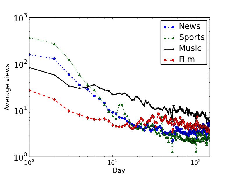
Figure 1: CDF of time-to-peak
videos experience relatively fewer views early in their of the peak views, defined as follows:
lifetime. Film videos follow an almost constant view-
ing rate for the entire measurement period. News and x = max(i) : view(i) ≥ 50% × view(peak) & i > peak
Sports videos, however, experience a significant por- (1)
tion of the total views early. where view(i) is the views on day i and view(peak)
is the number of views on the peak day. Only videos
with more than 100 views are considered. Figure 3
shows the peak day as a unique point in the lifetime
of videos for faster-growing categories (e.g., News
and Sports). These categories experience a popular-
ity burst, and quickly decline to a lower viewing rate.
Figure 2: Percent of total views over time
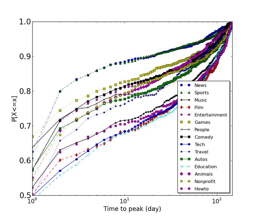
It is important to understand if the peak day differs
significantly from other days of a video’s lifetime in
order to determine if our previous statistic is helpful.
Figure 3 shows the complementary cumulative distri-
bution function (CCDF) of the most distant day x after
the peak such that the views on day x is at least 50% Figure 3: CCDF of time-after-peakMany Music, Film, Howto, Education and Tech
videos that reach peak popularity comparatively lately
do not have that drop in their popularity (Figures 1
and 3), so time to reach peak popularity is propor-
tional to the active lifespan of a video. For example,
over 75% of the News and Sports videos never ex-
perience half of their peak days’ views after the peak
day (Figure 3), but fewer than 50% for Film and Tech
videos have this characteristic. The stability of Film
and Tech videos suggests that a longer measurement
period would increase the difference between these
categories and News/Sports.
We are also interested to know if the categories
that reach peak popularity faster than others also ex-
perience differing numbers of views. Figure 4 depicts
the 95th percentile of views of all categories over time. Figure 4: 95th percentile of views per day
We show the 95th percentile to remove the potential
effect of outliers. This shows which categories have
a minimum percentage of popular videos (5%) during
the first 100 days of the data collection and the relative
popularity of the categories for those popular videos.
The last 49 days of the collection period are virtually
identical to days 50-99 in terms of this measure.
These graphs illustrate how viewing patterns
of different categories change throughout the early
part of their lifetimes. Although the most similar
dataset collected (Borghol et al., 2011) shows that
the views of Music category exceeds all other cate-
gories within their 8-month measurement period,3 our
dataset shows that popular News, and Sports videos
enjoy higher viewing rates than any other types of
videos for the first couple of days since publication.
Figure 4 suggests that almost all categories have at Figure 5: Time varying average added views
least 5% of their videos that experience a high ini-
tial viewing rate; the difference is that after these few
peak days, views for most of the categories become proximately 10% of the Music videos enjoy fewer
very low, except Music and to a lesser extent, Film than 10 views; this value is over 30% for Howto,
and Tech videos. The results indicate the variations in People, Autos, Comedy, and Travel. Music, News,
active life spans of different categories. Sports, and Film contain most of the popular videos
Although similar results can be observed from in our dataset (> 1.11% with over 10,000 views). The
the average views per day (Figure 5), this can be most unpopular videos are in the Travel category, fol-
misleading because of the high variance of views. lowed by Comedy and Animals. Only 0.44% of the
The higher early average views of Sports videos than People videos had more than 10,000 views, in spite
News videos is due to the most popular video in the of the highest uploading rate (shown later). Although
entire dataset, which happens to be a single enor- uploaders currently upload more UGC videos, users
mously popular Sports video with almost 24 times are still not attracted to UGC videos compared to
that of the second most popular Sports video. UCC (user copied content) videos.
4.2 Fractions of Popular Videos 4.3 Current Uploading Rate
The percent of videos with different views of the In order to design a request generator for YouTube,
YouTube categories are shown in Table 2. Only ap- it is important to know the category uploading rate.
In 2007, Music was in the top position in number
3 We collected category names of the videos which had of uploaded videos followed by Entertainment, Com-
not been deleted by running another crawler. edy, Sports and Film (Cheng et al., 2007). ManualTable 2: Percent of popular videos
Category ≤10 views 11 to 100 101 to 1000 1001 to 10000 10001 to 100000 > 100000
Pct Num Pct Num Pct Num Pct Num Pct Num Pct Num
Music 10.44 363 48.72 1694 32.87 1143 6.38 222 1.29 45 0.29 10
News 18.85 647 39.57 1358 31.61 1085 8.42 289 1.4 48 0.15 5
Sports 20.79 776 46.0 1717 26.12 975 5.97 223 1.04 39 0.08 3
Tech 22.56 605 47.28 1268 24.61 660 4.85 130 0.63 17 0.07 2
Film 23.06 541 49.53 1162 20.84 489 5.46 128 1.07 25 0.04 1
Entertainment 27.77 702 46.88 1185 20.61 521 3.88 98 0.75 19 0.12 3
Howto 43.79 776 34.59 613 17.04 302 4.01 71 0.45 8 0.11 2
Nonprofit 24.11 890 48.04 1773 23.49 867 3.85 142 0.46 17 0.05 2
Education 24.73 940 48.83 1856 21.7 825 4.34 165 0.37 14 0.03 1
Animals 25.59 1060 56.48 2340 15.52 643 2.05 85 0.34 14 0.02 1
Games 27.51 816 49.36 1464 19.08 566 3.44 102 0.51 15 0.1 3
People 29.52 806 49.93 1363 17.69 483 2.42 66 0.4 11 0.04 1
Autos 30.57 992 41.45 1345 23.17 752 4.07 132 0.68 22 0.06 2
Comedy 32.33 1121 51.08 1771 14.08 488 2.08 72 0.35 12 0.09 3
Travel 33.75 1248 48.89 1808 15.44 571 1.76 65 0.14 5 0.03 1
popular YouTube videos follow a Zipf-like distribu-
tion, a Weibull distribution fits better because of the
heavy tail section, which indicates a large number of
very unpopular videos in YouTube. After considering
video categories, only News videos follow a Weibull
distribution for the first 80% of the videos, because of
the comparatively flatter head section of News access
pattern. This is consistent with fetch-at-most-once be-
haviour (Gummadi et al., 2003), as would be expected
in watching news videos. For all other categories, re-
quest distributions of popular videos follow Zipf dis-
tributions and the heavy tail sections of the categories
can be fit with a Weibull cutoff, as can be seen with
the high goodness of fit statistic (R2 ). The number of
Figure 6: Category Uploading Rate (365,000 videos) videos that exhibit Zipf behaviour differs between the
categories, showing different-sized tails.
Another measure that we calculated was the
sampling revealed that these categories are dominated CCDF of total views over the measurement period.
by UCC rather than UGC, so most of the videos in There were a substantial number of videos in certain
YouTube were actually UCC. categories that had at most 1 view. This can skew the
Figure 6 shows the current uploading trend of popularity measures. The HowTo and Autos category
YouTube videos obtained by crawler 3. We see that had 17% and 12.6% of videos with at most 1 view,
the uploading trend in YouTube has changed over respectively, while 9% of HowTo videos had 0 views.
time. The People category is at the top position with There is a section of completely unpopular videos that
approximately 24% of all the new videos, which was get published, but never viewed. Figure 8 shows the
at the 6th position in 2007, only 8% of all the videos. CCDF of the total views for a selected number of cat-
Samples from the People category contain compara- egories. We truncate the x-axis to see the behaviour
tively more UGC objects than other categories. of views for unpopular videos more clearly. Enter-
tainment is used as an example of a group of cate-
4.4 Category Popularity Distributions gories that had very similar CCDFs (Entertainment,
Games, People, Education and Tech). The shape of
Figure 7 shows the Rank-frequency distribution for the distribution of total views is very similar in these
the 6 categories that showed the most interesting pat- categories, but that of views over time is not. Music
terns. Previous studies (Abhari and Soraya, 2010; has very few videos below 20 views, but HowTo has
Cheng et al., 2007) showed that although requests for almost 50% of the videos below 20 views.(a) News (b) Music (c) Entertainment
(d) Film (e) People (f) Comedy
Figure 7: Number of views against rank for categories
shots of the measurement period.
n ∑ xi yi − (∑ xi )(∑ yi )
rxy = q q (2)
n ∑ xi2 − (∑ xi )2 n ∑ y2i − (∑ yi )2
A high correlation coefficient between early views
and and the rest of the period implies that prediction
of future views of individual videos is achievable (Sz-
abo and Huberman, 2010). We got very encouraging
results for some of the categories including Sports,
Travel, Howto, Tech and Games.5
However, for other categories like Film, News,
Entertainment the coefficients are very poor, indi-
cating the significant changes in the set of popular
videos. Music shows a bit different characteristics
Figure 8: Selected CCDF of total views
though, if we take first 10 days as our first snapshot.
5 TOWARDS A WORKLOAD 5.2 Time-Series Clustering
GENERATOR This category variation led us to model the growth
patterns differently. Three-phase characterization
(Borghol et al., 2011), does not work for the cate-
5.1 Predicting Popularity gory specific modeling, as the number of videos that
are at or before their peak phases in a particular day
As an approach to predict future popularity of videos, are very different between first few days and last few
Pearson’s correlation coefficient (Equation 2) is cal- days in our measurement period. We thus decided to
culated between the added views4 at different snap- investigate whether the growth patterns of videos in
5 Sportsis 0.99 for the first day’s views and the rest of
4 Added views is the number of views on a particular day the measurement perioda specific category follow similar shapes. This ap- in each cluster differ between these two categories,
proach can be considered as a time-series clustering complementing our earlier findings. 46% of Music
problem and becomes a challenging problem as dif- videos are contained within the slower-decaying clus-
ferent videos reach peak popularity at different times. ters; this drops to 15% for News videos.
Inspired by a study on viral videos (Broxton et al., An important question that must be answered is
2010), we translate all the time-series so that the x- whether a particular cluster is more biased to popular
axis is centred on the peak day, since most of the sig- videos than others. This can be answered by taking
nificant events happen around the peak periods. the average of the rank values of all the videos in a
Another challenging issue is to select the appro- cluster. The central limit theorem suggests that the
priate time-series clustering algorithm. We are par-
ticularly interested to identify similar shapes of the
views per day, regardless of the time to peak. More-
over, the algorithm should not be affected much by
outliers. We selected K-SC clustering (Yang and
Leskovec, 2011), which has been found to be accurate
in identifying the growth patterns of other Web con-
tent. Unlike K-means clustering, K-SC cluster cen-
troids are not distorted by outliers. Instead of consid-
ering Euclidean distance between the curves, K-SC
applies a scale and shift invariant distance metric (Chu
and Wong, 1999). We evaluated the performance of
K-SC algorithm for only two categories: Music and
News. The clustering was performed only for the top
2000 videos in order to present more accurate results.
Figure 9 shows the six clusters for Music videos
found by K-SC. Forcing K-SC to select fewer than six Figure 10: News-clusters
clusters drops the accuracy significantly, as we lose
some of the interesting patterns. However, more than average rank of each cluster of videos should be 1000
six clusters does not significantly improve the accu- if it is not popularity-biased. For News videos, the
racy as we observe the repetition of similar clusters. average rank values are very similar for each cluster
(near 1000). For Music videos, the clusters with com-
paratively slower decay contain more popular videos,
with average rank values of approximately 700. Pop-
ular Music videos observed a sharp decay with less
frequency than popular News videos.
5.3 Performance of K-SC
In order to evaluate the performance of K-SC, we de-
signed a synthetic workload generator for News and
Music videos. The synthetic data should show simi-
lar characteristics to the empirical YouTube data if the
clustering of K-SC is accurate.
The workload generator can be described as fol-
lows. A rank value is assigned to each of the 2000
videos as suggested by the chosen distributions for
Figure 9: Music-clusters
Music and News respectively. Then centroid/cluster
The cluster shapes for News videos (Figure 10) is assigned to the videos based on the distribution we
are very similar to Music (except very little differ- observed earlier. We also imposed a little bias for
ence between cluster (a) and (e) in Figures 9 and the popular videos before selecting the appropriate
10 respectively).6 However, the numbers of videos cluster in order to match our observed average rank
value. Although for News videos the time-to-peak
6 matching clusters are not in the same position in the distributions are very similar for each of the clusters,
graphs we found very different results for Music videos, asshown in Figure 11. We consider these peak distribu-
tions separately in our request generator.
Figure 13: Popularity distributions
6 CONCLUSIONS AND FUTURE
Figure 11: Peak distribution for music videos
WORK
We test similarity between the synthetic and em-
pirical data from four different perspectives: 1) The
In this paper, we analyzed global daily viewing pat-
total view distribution, 2) time-to-peak distribution, 3)
terns of a representative subset of YouTube videos
Average daily views over time, and 4) 95th percentile
from their time of publication until they were 5
of views over time.
months old. We discovered significant time-varying
Figures 12 and 13 indicate very good matches
popularity differences between categories.
between synthetic and empirical data for metrics 1
and 2, which does not in itself indicate high ac- Most videos exhibit their peak viewing day very
curacy of K-SC. We imposed the distributions for soon after publication and then there is a decay; rel-
these two cases from our observations, i.e., fixed atively few videos ever return to near their peak pop-
peak and Zipf/weibull distributions. Metrics 3 and 4 ularity. We determined that video categories which
show, however, that the clusters found by K-SC algo- reached their peaks later were more stable. This is ex-
rithm for both categories represent most of the videos pected and matches our intuitions. We developed an
growth patterns (Figure 14 and 15, respectively). analysis method that permits quantification of these
differences on a particular dataset. The confirmation
of Zipf distributions for the total views of popular
videos in nearly every category indicates that caching
would be effective.
We were also able to determine the relative trends
of viewing patterns of videos within categories over
the first few months of their lifetimes. Some cate-
gories contain a non-trivial number of videos which
are still popular 5 months after upload date, whereas
other categories have viewing patterns which dwin-
dle to nothing. Some categories have videos which
exhibit stationary behaviour that allows prediction of
which videos will remain relatively popular based on
their early views. Popularity changes around peak
time can be captured by appropriate time-series clus-
Figure 12: Time-to-peak distributions tering. While we use a dataset from YouTube, issues
regarding the scale and deployment make direct ap-
Similar daily average views on a particular day in- plicability to YouTube impractical. Multiple regional
dicates that view distribution among videos on that caches are needed to satisfy the demand and regional
particular day are similar both in the empirical and differences (Brodersen et al., 2012). Our methodol-
synthetic data. These results show a smaller number ogy and analysis could be used to help design, con-
of outliers in both of the categories. figure, and deploy any category specific UGC site.Broxton, T., Interian, Y., Vaver, J., and Wattenhofer, M.
(2010). Catching a viral video. In IEEE Data Min-
ing Workshops, pages 296–304, Sydney, Australia.
Cha, M., Kwok, H., Rodriguez, P., Ahn, Y., and Moon, S.
(2009). Analyzing the Video Popularity Characteris-
tics of Large-Scale User Generated Content Systems.
IEEE/ACM Trans. Netw., 17(5):1357–1370.
Cheng, X., Dale, C., and Liu, J. (2007). Understanding
the Characteristics of Internet Short Video Sharing:
YouTube as a Case Study. Technical report, Cornell
University, arXiv e-prints.
Chu, K. K. W. and Wong, M. H. (1999). Fast time-series
searching with scaling and shifting. In ACM PODS
1999, pages 237–248, Philadelphia, PA.
Ding, Y., Du, Y., Hu, Y., Liu, Z., Wang, L., Ross, K., and
Figure 14: Daily views over time Ghose, A. (2011). Broadcast Yourself: Understanding
YouTube Uploaders. In ACM IMC 2011, pages 361–
370, Berlin, Germany.
Figueiredo, F., Benevenuto, F., and Almeida, J. (2011). The
Tube over Time: Characterizing Popularity Growth of
Youtube Videos. In ACM WSDM 2011, pages 745–
754, Hong Kong, China.
Gember, A., Anand, A., and Akella, A. (2011). A Compar-
ative Study of Handheld and Non-handheld Traffic in
Campus Wi-Fi Networks. In PAM 2011, pages 173–
183, Atlanta, GA.
Gill, P., Arlitt, M., Li, Z., and Mahanti, A. (2007). Youtube
Traffic Characterization: A View From the Edge. In
ACM IMC 2007, pages 15–28, San Diego, CA.
Gummadi, K. P., Dunn, R. J., Saroiu, S., Gribble, S. D.,
Levy, H. M., and Zahorjan, J. (2003). Measure-
ment, modeling, and analysis of a peer-to-peer file-
sharing workload. In ACM SOSP 2003, pages 314–
Figure 15: 95th percentile of views over time 329, Bolton Landing, NY.
Khemmarat, S., Zhou, R., Gao, L., and Zink, M. (2011).
Watching User Generated Videos with Prefetching. In
As future work, we are in the process of building a ACM MMSYS 2011, pages 187–198, San Jose, CA.
complete workload generator that encompasses more
Labovitz, C., Iekel-Johnson, S., McPherson, D., Oberheide,
aspects of user-generated content video requests. In J., and Jahanian, F. (2010). Internet Inter-Domain
particular, we will incorporate category-specific in- Traffic. In ACM SIGCOMM 2010, pages 75–86, New
troduction of new content over time to drive simula- Delhi, India.
tions and/or prototype content distribution networks Maier, G., Schneider, F., and Feldmann, A. (2010). A First
to evaluate different design policies for storing and Look at Mobile Hand-held Device Traffic. In PAM
delivering videos. 2010, pages 161–170, Zurich, Switzerland.
Siersdorfer, S., Chelaru, S., Nejdl, W., and Pedro, J. S.
(2010). How Useful are Your Comments?: Analyz-
ing and Predicting YouTube Comments and Comment
REFERENCES Ratings. In World-Wide Web 2010, pages 891–900,
Raleigh, NC.
Abhari, A. and Soraya, M. (2010). Workload Generation Szabo, G. and Huberman, B. (2010). Predicting the popu-
for YouTube. Multimedia Tools and Applications, larity of online content. CACM, 53(8):80–88.
46(1):91–118. Yang, J. and Leskovec, J. (2011). Patterns of temporal vari-
Borghol, Y., Mitra, S., Ardon, S., Carlsson, N., Eager, D., ation in online media. In ACM WSDM 2011, pages
and Mahanti, A. (2011). Characterizing and Mod- 177–186, Hong Kong, China.
elling Popularity of User-Generated Videos. Perfor- Zink, M., Suh, K., Gu, Y., and Kurose, J. (2009). Char-
mance Evaluation, 68:1037–1055. acteristics of YouTube Network Traffic at a Campus
Brodersen, A., Scellato, S., and Wattenhofer, M. (2012). Network - Measurements, Models, and Implications.
YouTube Around the World: Geographic Popularity Computer Networks, 53(4):501–514.
of Videos. In World-Wide Web 2012, pages 241–250,
Lyon, France.You can also read