Prediction of Price Increase for Magic: The Gathering Cards
←
→
Page content transcription
If your browser does not render page correctly, please read the page content below
Prediction of Price Increase for Magic: The Gathering
                              Cards

         Matthew Pawlicki                         Joseph Polin                        Jesse Zhang
     Aeronautics and Astronautics              Computer Science                   Electrical Engineering
         Stanford University                   Stanford University                 Stanford University
    pawlick9@stanford.edu                   jpolin@stanford.edu                 jessez@stanford.edu

                                                   Abstract

         Magic: The Gathering (MTG) is a trading card game that drives an extensive second-hand
         market. Given the relatively high price and traffic volume of these cards, there is motivation to
         investigate the parameters of the market with the hope of predicting its behavior. Specifically,
         this study aimed to use historical price, sales, and tournament-usage data to predict dramatic,
         short-term price changes in specific cards. Classification algorithms, such as logistic regres-
         sion and support vector machines, proved effective in anticipating such price changes. On
         average, investing in cards using the models detailed in this report would theoretically lead
         to a substantial net profit.

1   Background and Motivation

Magic: The Gathering is a successful trading card game with roots going back to 1993. The active MTG
community is composed of over 12 million players around the world and continues to grow at a rapid pace
[1]. The game itself is highly strategic and requires players to acquire and maintain carefully crafted decks
of at least sixty cards. With tournaments paying out upwards of $250,000 [2], active players often spend
close to $1,000 annually curating decks that suit their strategies. The contents of tournament-winning decks
are posted publicly and tend to influence the dominant and popular strategies at any given time. Players may
purchase packs of randomly assorted cards from major retailers as well as single cards available at card shops
or online vendors in the secondary market. The combination of a strong and growing MTG community, well-
defined strategy influences, and the availability of secondary market data permits a legitimate opportunity for a
machine learning price prediction study.

2   Data

The raw data set included card price history, tournament usage, sales volume history, and the intrinsic attributes
for each card. The tournament usage data was extracted from MTGtop8.com which publishes the contents
of tournament-winning decks from around the world. The price and sales volume history, which drew from
thousands of vendors around the country, was provided by a developer at MTGprice.com, a website dedicated
to compiling this sort of data. Card attributes were obtained from MTGjson.com, a free card database API.
Each sample of the data set represented a specific card on a specific date. Samples missing price, usage, or
attribute data were omitted. Further, only cards whose rarity (a denotation assigned by the card manufacturer)
was Rare or Mythic Rare were included since these tend to be more expensive and exhibit higher potential
gains. Ultimately, the data set consisted of m = 13,608 samples, all of which were from May 2012 through
August 2014.

                                                        1
3 Feature and Label Selection
Each sample pertained to information for a specific card K on a specific date D and included the 28 features
shown in Table 3. The expression for usage of card K on date D in tournament-winning decks is given by:
K # times card K was used from date D − 6 through date D
UD = (1)
Total # of cards used from date D − 6 through date D
Table 1: Selected Features for card K on date D
Indices Feature(s) Description
K K K
1-7 PD , PD−1 , ... , PD−6 Prices for day D and preceding week
8 - 13 K
(PD K
− PD−1 K
), (PD K
− PD−2 K
), ..., (PD K
− PD−6 ) Price difference between day D and each of
the previous 6 days
14 - 19 K
(UD K
− UD−1 K
), (UD K
− UD−2 K
), ..., (UD K
− UD−6 ) Usage difference between day D and each of
the previous 6 days
K K K K K K Sales volume difference between day D and
20 - 25 (SD − SD−1 ), (SD − SD−2 ), ..., (SD − SD−6 ) each of the previous 6 days.
26 MK Converted mana cost attribute
K
27 RD Days until card loses tournament legality
2 K
28 (σD ) Variance of past week’s prices
In attempts to improve the performance of the classification algorithms mentioned in section 4, the time-
dependent features (price, usage, and sales volume) were low-pass filtered and normalized to generate modified
data sets. The full data set was also divided into smaller sets by clustering on card type, such as ”Creature” or
”Enchantment” (7 types total), or removing samples whose average daily price never exceeded a certain price
threshold.
Labelings were constructed as binary classifications in an effort to detect profitable, investible situations. Four
different labeling were considered, as shown in Table 3. The inclusion of a $0.50 margin in labelings 3 and 4
were intended to structure a profit margin into the classification that would offset transactional costs such as
postage upon resale.
Table 2: Various labeling schemes considered
Index Labeling Scheme Description
1
K
y i = 1 PD K
< P̄D+1:D+7 True if price on day D is less than average price
over following week
K K True if price on day D is less than minimum
2 y i = 1 PD < minD0 :D+1≤D0 ≤D+7 PD 0
price over following week
K K True if price on day D is at least $0.50 less than
3 y i = 1 PD + $0.50 < P̄D+1:D+7 average price over following week
K K True if price on day D is at least $0.50 less than
4 y i = 1 PD + $0.50 < minD0 :D+1≤D0 ≤D+7 PD 0
minimum price over following week
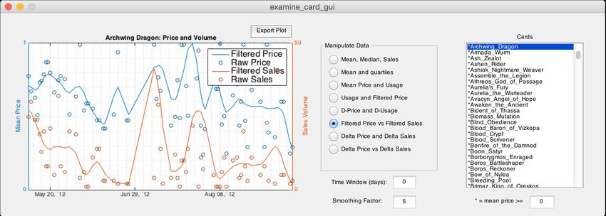
As a means for visualizing price, sales, and tournament usage metrics over time, a custom MATLAB graphical
user interface (GUI) was developed (see Figure 1). The GUI allowed for the variation of parameters such as
filter coefficient, price threshold, and time window. This tool proved helpful in determining useful features and
gaining an intuition for how MTG card prices were affected by usage and sales volume.
2Figure 1: Custom-designed graphical user interface for examining price data
4 Model Selection
Given that the primary goal of the study was posed as a binary classification problem designed for determining
whether or not to buy a card on a specific date, classification algorithms such as logistic regression (LR) and
support vector machine (SVM) were deemed most appropriate. After initial classification attempts, the data set
was discovered to not be linearly separable, and regularization techniques were used to improve the robustness
of each model. Both models were tested using a k-fold cross validation implementation to minimize the effects
of exceptional trials.
4.1 Logistic Regression
Regularized LR was implemented according to equations 2 through 4 based on [3]. For the sake of comparison,
both L1 and L2 regularization were tested. The results from the LIBLINEAR [4] L2 -regularized LR code was
confirmed with an independently developed MATLAB implementation.
m
X
θ = arg max log p(y (i) |x(i) ; θ) + λ||θ||2 (2)
θ i=1
(i) (i)
p(y (i) |x(i) ; θ) = h(θT x(i) )y (1 − h(θT x(i) ))1−y (3)
T (i) 1
h(θ x ) = 1 > 0.5 (4)
1 + e−θT x(i)
For the L2 -regularized LR, the theta vector was derived using batch gradient descent whose update rule is
given by Equations 5 and 6. In these expressions, α is the learning rate, λ is the regularization parameter, and j
(i)
subscript corresponds to the j th element of an (n + 1) × 1 vector. Note that xo = 1 and serves as the intercept
term.
m
1 X
θo := θo − α (h(θT x(i) ) − y (i) )xo(i) (5)
m i=1
m
1 X (i) λ
θj := θj − α (h(θT x(i) ) − y (i) )xj ) + θj (6)
m i=1 m
34.2 Support Vector Machine
A regularized SVM was implemented according to Equations 7 and 8 where θ = [b wT ]T holds the parameters
that SVM attempts to determine and C, ranging from 0.1 to 100, is the weight applied to the regularization
term. The L1 and L2 norms were considered for both the objective and loss terms.
n o
h(θT x(i) ) = 1 wT x(i) + b > 0 (7)
m
1 X 2
w = min ||w||2 + C max(0, 1 − y (i) w, x(i) (8)
w 2
i=1
4.3 Performance Metrics
To evaluate the performance of the LR and SVM approaches, several metrics were considered. First, the
classification errors (sum of false positives and false negatives divided by m) of the models were compared
to the classification error obtained from the trivial classifier, which labeled all samples 0 (never buy). After
outperforming the trivial classifier, performance was evaluated using the likelihood ratio, L, or the ratio of the
true positive rate (TPR) to the false positive rate (FPR). Since true positives and false positives were the only
scenarios in which money was made or lost, there was justifiable motivation to maximize this ratio.
Although the models were meant to maximize the percentage of correct buy/don’t-buy decisions, a real-world
application would be concerned most about maximizing the profit obtained. Thus, models were further evalu-
ated based on the amount of profit generated per buy, the amount of profit generated per card in the data set, the
return on investment (ROI), and the percentage of maximum possible profit. Ultimately, percent-error, e, and
percentage of maximum possible profit, f , were selected to be the primary metrics by which various models
were assessed.
m
1 X (i) (i)
f (θ) = h(θT x(i) ) µd − Pd (9)
prof itmax i=1
m n o
(i) (i) (i) (i)
X
prof itmax = 1 µd − Pd > 0 µd − Pd (10)
i=1
5 Results
Filtering the time-dependent data decreased the performance of all models, and normalizing the data sets re-
sulted in marginal improvement. Clustering by card type and removing low-price cards resulted in data sets
that were too small to yield consistent models. The labeling corresponding to a change in mean price exceeding
$0.50 produced the best results for both accuracy and percentage of maximum possible profit recovered (see
Table 5).
Table 3: Classification results
Model Training Set (m=10,213) Testing Set (m=3,405)
SVM e = 15% f = 85% e = 15% f = 85%
LR e = 12% f = 88% e = 11% f = 93%
75% of the data set was used for training and 25% was used for testing. The classification error is given by
e and the percentage of maximum possible profit, f , is given in equation 9. The data was labeled using label
3 in Table 3. Using forward search, UD − UD−3 (feature 16 in Table 3) generated the highest percentage of
maximum profit, and SD − SD−3 (feature 22) generated the greatest true-positive to false-positive ratio.
46 Discussion
Although SVM and LR both produced positive profits, LR yielded the highest f with the lowest e. This may
be because rather than creating the optimal separation between the closest samples (the support vectors, in the
case of SVM), LR factors in a degree of confidence that correlates to price difference (see Figure 2).
30
Recommend DON'T BUY
20 Recommend BUY
10
µd-Pd
0
-10
-20
-30
-1.5 -1 -0.5 0 0.5 1
θTx ×10 5
Figure 2: Price change vs feature weighting for logistic regression
Of the 28 features used, the variance of the past week’s prices and the converted mana cost of a card contributed
the least. As expected, changes in price, usage, and sales volumes especially within 3 days of the current day
were the greatest indicators for upcoming price trends.
7 Future Work
A logical next step to improving the models would be to more thoroughly evaluate the performance metrics.
Recasting these metrics as convex optimization problems and maximizing them would result in models that
prioritize generating profit over simply being accurate. Also, it would be worthwhile to consider the impact of
other factors inherent to a real-world implementation, such as transaction logistics, trading of multiple copies
of the same card, and strategies for re-sale. Also, the time frame over which the price was predicted was fixed
at a week. This time frame was likely sub-optimal and presents an avenue for further investigation.
8 Acknowledgments
We would like to thank MTGtop8.com, for providing us the data for the tournament deck lists, MTGjson.
com, for providing us the card database API, and Alasdair Young from MTGprice.com, for providing us the
price and vendor inventory data from May 2012 to August 2014. We would also like to thank Andrew Ng and
all of the CS 229 teaching assistants for their mentorship and guidance this quarter.
References
[1] Y. LeJacq. (2013, August) At 20, magic:the gathering still going strong. [Online]. Available:
http://www.nbcnews.com/
[2] (2013, February) Pro tour gatecrash event information.
[3] A. Y. Ng, “Logistic regression,” 2014.
[4] R.-E. Fan, K.-W. Chang, C.-J. Hsieh, X.-R. Wang, and C.-J. Lin, “Liblinear: A library for large linear
classification,” The Journal of Machine Learning Research, vol. 9, pp. 1871–1874, 2008.
5You can also read