Prediction of Wine Quality Using Machine Learning Algorithms
←
→
Page content transcription
If your browser does not render page correctly, please read the page content below
Open Journal of Statistics, 2021, 11, 278-289
                                                                                                https://www.scirp.org/journal/ojs
                                                                                                            ISSN Online: 2161-7198
                                                                                                              ISSN Print: 2161-718X

Prediction of Wine Quality Using Machine
Learning Algorithms

K. R. Dahal1*, J. N. Dahal2, H. Banjade3, S. Gaire4
1
  Department of Statistics, Truman State University, Kirksville, MO, USA
2
  Department of Physics, Virginia Union University, Richmond, VA, USA
3
  Department of Physics, Virginia Commonwealth University, Richmond, VA, USA
4
  Department of Physics, The Catholic University of America, Washington D. C., USA

How to cite this paper: Dahal, K.R., Dah-       Abstract
al, J.N., Banjade, H. and Gaire, S. (2021)
Prediction of Wine Quality Using Machine        As a subfield of Artificial Intelligence (AI), Machine Learning (ML) aims to
Learning Algorithms. Open Journal of Sta-       understand the structure of the data and fit it into models, which later can be
tistics, 11, 278-289.
                                                used in unseen data to achieve the desired task. ML has been widely used in
https://doi.org/10.4236/ojs.2021.112015
                                                various sectors such as in Businesses, Medicine, Astrophysics, and many oth-
Received: February 9, 2021                      er scientific problems. Inspired by the success of ML in different sectors, here,
Accepted: March 15, 2021                        we use it to predict the wine quality based on the various parameters. Among
Published: March 18, 2021
                                                various ML models, we compare the performance of Ridge Regression (RR),
Copyright © 2021 by author(s) and               Support Vector Machine (SVM), Gradient Boosting Regressor (GBR), and
Scientific Research Publishing Inc.             multi-layer Artificial Neural Network (ANN) to predict the wine quality.
This work is licensed under the Creative
                                                Multiple parameters that determine the wine quality are analyzed. Our analy-
Commons Attribution International
License (CC BY 4.0).                            sis shows that GBR surpasses all other models’ performance with MSE, R, and
http://creativecommons.org/licenses/by/4.0/     MAPE of 0.3741, 0.6057, and 0.0873 respectively. This work demonstrates,
               Open Access                      how statistical analysis can be used to identify the components that mainly
                                                control the wine quality prior to the production. This will help wine manu-
                                                facturer to control the quality prior to the wine production.

                                                Keywords
                                                Wine Quality, Neural Network, Machine Learning (ML), Artificial
                                                Intelligence (AI)

                                              1. Introduction
                                              Wine is the most commonly used beverage globally, and its values are consi-
                                              dered important in society. Quality of the wine is always important for its con-
                                              sumers, and mainly for producers in the present competitive market to raise the

DOI: 10.4236/ojs.2021.112015       Mar. 18, 2021                  278                                     Open Journal of Statistics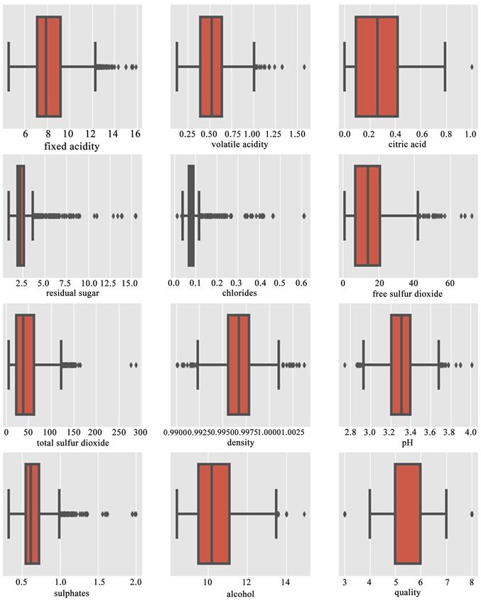
K. R. Dahal et al.

                               revenue. Historically, wine quality used to be determined by testing at the end of
                               the production; to reach that level, one already spends lots of time and money. If
                               the quality is not good, then the various procedure needs to be implemented
                               from the beginning, which is very costly. Every person has their own opinion
                               about the taste, so identifying a quality based on a person’s taste is challenging.
                               With the development of technology, the manufacturers started to rely on vari-
                               ous devices for testing in development phases. So, they can have a better idea
                               about wine quality, which, of course, saves lots of money and time. In addition,
                               this helped in accumulating lots of data with various parameters such as quantity
                               of different chemicals and temperature used during the production, and the
                               quality of the wine produced. These data are available in various databases (UCL
                               Machine Learning Repository, and Kaggle). With the rise of ML techniques and
                               their success in the past decade, there have been various efforts in determining
                               wine quality by using the available data [1] [2] [3]. During this process, one can
                               tune the parameters that directly control the wine quality. This gives the manu-
                               facturer a better idea to tune the wine quality by tuning different parameters in
                               the development process. Besides, this may result in wines with multiple tastes,
                               and at last, may result in a new brand. Hence, the analysis of the basic parame-
                               ters that determine the wine quality is essential. In addition to humanitarian ef-
                               forts, ML can be an alternative to identify the most important parameters that
                               control the wine quality. In this work, we have shown how ML can be used to
                               identify the best parameter on which the wine quality depends and in turn pre-
                               dict wine quality.
                                 Our work is organized as follows: In Section 2, we discuss data description
                               and preprocessing of the dataset used in this work. In Section 3, we briefly dis-
                               cuss the proposed methodology, followed by model comparison and selection of
                               best model in Section 4. In Section 5, we summarize the main finding and con-
                               clusion.

                               2. Data Description and Preprocessing
                               2.1. Data Source and Description
                               In this study, we use the publicly available wine quality dataset obtained from
                               the UCL Machine Learning Repository, which contains a large collection of
                               datasets that have been widely used by the machine learning community [4].
                               Among the two types of wine quality dataset (redwine and white wine), we
                               have chosen redwine data for our study because of its popularity over the
                               white wine. The redwine dataset contains 11 physiochemical properties: fixed acidi-
                               ty (g[tartaric acid]/dm3),volatile acidity (g[acetic acid]/dm3), total sulfur dioxide
                               (mg/dm3), chlorides (g[sodium chloride]/dm3), pH level, free sulfur dioxide
                               (mg/dm3), density (g/cm3), residual sugar (g/dm3), citric acid (g/dm3), sulphates
                               (g[potassium sulphate]/dm3), and alcohol (vol%). Alongside these properties, a
                               sensory score was acquired from several different blind taste testers which graded
                               each wine sample with a score ranging from zero (poor) to 10 (excellent). The

DOI: 10.4236/ojs.2021.112015                        279                                    Open Journal of Statistics
K. R. Dahal et al.

                               median was recorded and serves as the response variable [5]. The dataset con-
                               tains the records of 4898 random samples of wine manufactured. Various statis-
                               tical analyses were done to understand the nature of the dataset as presented in
                               Table 1.
                                  The Pearson correlation coefficient (r) measures the strength of the associa-
                               tion between two different variables. The association between two variables is
                               considered highly positive if ‘r’ is close to 1 while highly negative if “r” is close to
                               −1. Before passing the data into the ML models, we calculated the Pearson cor-
                               relation coefficient between each variable and the wine quality (i.e., target prop-
                               erty) in our dataset, as presented in Table 2. Our analysis shows that quantity of
                               alcohol has the highest (0.435), while the citric acid has the lowest (−0.009) cor-
                               relation coefficients with the target property. The variables which have the sig-
                               nificantly lower correlation coefficient (close to zero) with the target property
                               can be considered as irrelevant in the statistical analysis. While training the ML
                               models these variables can have significant effect in the predicted property, as
                               they introduced the noise in the dataset and mislead the training process. This
                               results in poor models and less accurate prediction performance. There are dif-
                               ferent ways to decrease noise [6]. One of the most popular and commonly used
                               methods of denoising is dropping the irrelevant, redundant, and insignificant
                               predictors. The method, which is simple, and convenient comes first in the mind
                               of a statistician [7] [8].
                                  ML algorithms are sensitive to the outliers. It can spoil and mislead the train-
                               ing process. As a result, we may end up with poor models which ultimately give
                               less accurate results. So, it is customary to check outliers during the data pre-
                               processing. A boxplot is a standardized way of displaying the distribution of the

                               Table 1. Descriptive statistics of the variables of the redwine data.

                                                                         Standard
                                     Variable Name              Mean                   Minimum         Maximum     Median
                                                                         deviation

                                       Fixed acidity            6.854      0.843          3.80           14.2        6.80

                                     Volatile acidity           0.278      0.100          0.08           1.10        0.26

                                        Citric acid             0.334      0.121          0.00           1.66        0.32

                                      Residual sugar            6.391      5.072          0.60           65.8        5.20

                                        Chlorides               0.045      0.021          0.009          0.35        0.04

                                    Free sulfur dioxide         35.30      17.00          2.00           289         34.0

                                   Total sulfur dioxide         138.4      42.49          9.00           440         134

                                          Density               0.994      0.002          0.99          1.038        0.99

                                            PH                  3.188      0.151          2.27           3.82        3.18

                                        Sulphates               0.489      0.114          0.22           1.08        0.47

                                          Alcohol               10.51      1.230          8.00           14.2        10.4

                                          Quality               5.877      0.885          3.00           9.00        6.00

DOI: 10.4236/ojs.2021.112015                              280                                     Open Journal of Statistics
K. R. Dahal et al.

                               Table 2. The value of the pearson correlation coefficient (r) of the predictors with respect
                               to the target variable: quality.

                                       Predictor         r          Predictor            r         Predictor           r

                                       Alcohol         0.435        Citric acid       −0.009     Volatile acidity   −0.194

                                          pH           0.099      Residual sugar      −0.097        Chlorides       −0.209

                                       Sulphates       0.053       Fixed acidity      −0.113        Density         −0.307

                                 Free sulfur dioxide   0.008   Total sulfur dioxide   −0.174

                               data. It is commonly used to identify the shape of the distribution and the possi-
                               ble existence of the outliers. Boxplots of each feature are plotted in Figure 1.
                               Based on these boxplots, all the variables except alcohol are either skewed or
                               possibly contain outliers. To get rid of outliers, we may drop the extreme values
                               from the data set. However, dropping data is always a harsh step, so should be
                               taken only in the extreme condition when we are 100 % sure that the outliers are
                               the measurement errors. At this point, we are unable to drop these extreme val-
                               ues because we are unable to confirm these extreme values as measurement er-
                               rors.

                               2.2. Feature Scaling
                               As presented in Table 1, the variables are spread widely. For instance, the values
                               of total Sulphur dioxide are extremely large compared to the chlorides. Such a
                               large value of one variable can have dominance over other quantities during the
                               training process in ML models. For instance, while doing K-nearest neighbor
                               KNN [9], or SVM if one does not standardize the nonuniform data, the data-
                               points with high distance will dominate the performance of the KNN or SVM
                               model. So, feature scaling is a very important step one need to take care of, be-
                               fore training any ML model. There are many feature scaling methods. The most
                               common and popular techniques that have been using in the ML community are
                               standardization and normalization. There is not theoretical evidence of claiming
                               which method work best. To scale the features of the dataset, standardization has
                               been used. The formulas used to calculate the standardization is as follows:
                                                                        x − mean
                                                                   z=                                                      (1)
                                                                           std
                               where z, x, mean, and std are standardized input, input, mean and standard dev-
                               iation of the feature, respectively.

                               2.3. Data Partition
                               The data was split into training data set and testing data set in the ratio 3:1. We
                               train data and is used to find the relationship between target and predictor va-
                               riables. The main purpose of the splitting data is to avoid overfitting. If overfit-
                               ting occurs, the machine learning algorithm could perform exceptionally in the
                               training dataset, but perform poorly in the testing dataset [10].

DOI: 10.4236/ojs.2021.112015                           281                                      Open Journal of Statistics
K. R. Dahal et al.
Figure 1. Box plot of the variables of the redwine data.
3. Machine Learning Algorithms
A wide range of machine learning algorithms such as linear regression, logistic
regression, support vector machine, and kernel methods, neural networks, and
many others are available for the learning process [11]. Each technique has its
strength and weakness. In this work, we use the following supervised learning
algorithms to predict wine quality.
3.1. Ridge Regression
Ridge Regression (RR) is very similar to the multiple linear regression. In the mul-
tiple linear regression, the parameters β j are estimated by minimizing residual
sum of squares (RSS) defined in Equation (2).
(( y − β ))
2
= ∑ −∑ β j xij (2)
n p
RSS
=i 1 =
i 0 j 1
where yi are the observed value, and xij are the predictors.
DOI: 10.4236/ojs.2021.112015 282 Open Journal of StatisticsK. R. Dahal et al.
In the RR, the parameters are β j , the values that minimizes
(( y − β ))
2
∑ −∑ β x + λ∑ = RSS + λ ∑ j 1 β j2
β j2= (3)
n p p p
=i 1 =
i 0 j 1 =
j ij j 1
where λ ∑ j =1 β 2j is called the shrinkage penalty and λ is the tuning parameter
p
of the model [12]. When λ = 0, the RR is the same as linear regression because of
having common parameters. For the small value of λ, there is not a significant
difference between the parameters of the models. As λ increases, the parameters
of the RR started to shrink and converge to zero as λ → ∞ . The value of λ plays
a crucial role in the model performance. When λ is small there is high variance
and low bias; the model outperforms in the training set, while it has poor per-
formance in the unseen data, which results in overfitting. When λ increase, the
variance decreased, and the bias increases. For the sufficient high value of λ,
there might be underfitting, so a good choice of λ can have a best model, with
best prediction performance.
3.2. Support Vector Machine
Support Vector Machine (SVM) is one of the most popular and powerful ma-
chine learning algorithms which was introduced in the early 90s. When used for
regression, SVM is also known as Support Vector Regressor (SVR). SVR is a
kernel-based regression technique which maps nonlinearly separable data in real
space to higher dimension space using kernel function [13]. It is equipped with
various kernels such as linear, sigmoid, radial, and polynomial. In this work, we
have used radial basis kernel (RBF) because it outperformed other kernels based
SVR in redwine dataset. The performance of the SVR is controlled by two im-
portant tuning parameters (cost: regularization parameter and gamma: kernel
coefficient for RBF). The tuning parameter cost control the bias and variance
trade-off. The small value of the tuning parameters cost underfits the data, whe-
reas the large value overfit [12].
3.3. Gradient Boosting Regressor
Gradient Boosting Regression (GBR) is one of the leading ensemble algorithms
used for both classification and regression problems. Which builds an ensemble
of weak learners in sequence with each tree and together make an accurate pre-
dictor. Decision tree is one of the most popular choice of such ensemble models.
Each new tree added to the ensemble model (combination of all the previous
tree) minimize the loss function associated with the ensemble model. The loss
function depends on the type of the task performed and can be chosen by the
user. For GBR, the standard choice is the squared loss. A key factor of this model
is that adding sequentially trees that minimize the loss function, the overall pre-
diction error decreases [14] [15]. By tuning many hyperparameters such as the
learning rate, the number of trees, maximum depth we can control the gradient
boosting performance which helps to make model fast and less complex. De-
tailed explanation of the GBR algorithm can be found in Friedman et al. [14].
DOI: 10.4236/ojs.2021.112015 283 Open Journal of StatisticsK. R. Dahal et al.
3.4. Artificial Neural Network (ANNs)
ANNs are a very primitive generalization of biological neurons. They are com-
posed of layers of computational units called neurons, with a connection be-
tween different layers through the adjustable weights. The major constituents of
ANNs are weights, bias, and the activation function. An excellent choice of the
activation function results in the proper accuracy of an ANN model. The most
widely used activation functions are Logistic (known as Sigmoid) [16] [17] Rec-
tified linear unit, [18] and the SoftPlus [19]. Passage of information along a pre-
determined path between the neurons is the fundamental idea behind the con-
struction of ANNs. Its architecture is very flexible, and various network para-
meters (such as weights, bias, number of nodes, and number of hidden layers)
can be tuned to improve the performance of the network. One can add up the
information from multiple sources to the neurons and apply a non-linear trans-
formation at each node, which helps the network to learn the complexity present
in the data. With the application of linear and non-linear transformation in the
input data, ANNs transform those initial representations up to a specific out-
come. Depending on the learning task, the outcome of the network could be ei-
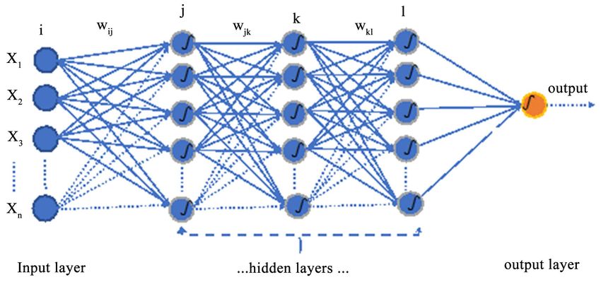
ther classification or regression. The schematic diagram for the ANN used in
this work is presented in Figure 2.
4. Results and Discussion
With the goal of assessing the performance of the different ML algorithms, we
have used four most popular machine learning algorithms, namely: Ridge Regres-
sion (RR), Support Vector Machine (SVM), Gradient Boosting Regressor (GBR),
and Artificial Neural Network (ANN) to predict the wine quality in the redwine
data. This allows us the freedom to select the most suitable ML algorithm to pre-
dict the wine quality with the given variables.
All of the model’s performance (on the training and test data) explained in the
previous sections are evaluated by using Mean Squared Error (MSE), Mean Ab-
solute Percentage Error (MAPE), and correlation coefficient (R) defined as
Figure 2. The schematic of an ANN, with three hidden layers and one output layer with
Relu activation function at each node where wij , wjk , and wkl are the weights.
DOI: 10.4236/ojs.2021.112015 284 Open Journal of StatisticsK. R. Dahal et al.
1 n
(
∑ yi − yi )
2
=
MSE (4)
n i =1
1 n yi − yi
MAPE = ∑
n i =1 yi
(5)
R=
∑ i =1 ( yi − yi )
n
( y − y )i i
(6)
( y − y ) ( y − y )
2 2
∑ i =1
n
i i i i
where, yi and yi are the target observed and target predicted values respec-
tively. And n is the total number of observations.
The 10-fold cross-validation is used to choose the best tuning parameter λ for
the RR model. We used the grid search technique to obtain the optimal parame-
ter by varying λ from 0.00001 to 100 with an increment of 0.01. Figure 3 shows
the variation in MSE with λ. We obtained the optimal value of λ as 45.25, that
minimizes the MSE. A RR model using this tuning parameter λ is fitted, and its
performance is presented in Table 3.
In addition to the RR, the performance of the kernel-based machine learning
algorithm SVM is compared. Similar to RR, the 10-fold cross-validation is used
to obtain the tuning parameters cost and gamma. We used the grid search tech-
nique to obtain these tuning parameters by varying each between 0.01 to 10. For
each possible combination of cost and gamma, MSE is computed. A heatmap of
Figure 3. Graph of tuning parameter λ versus the Mean squared error (MSE) of the RR
model.
Table 3. Model performance metrics obtained using training and test datasets.
Training data set Test data set
Models
R MSE MAPE R MSE MAPE
RR 0.6029 0.4281 0.0934 0.5897 0.3869 0.0888
SVM 0.7797 0.267 0.1426 0.5971 0.3862 0.1355
GBR 0.7255 0.3286 0.0826 0.6057 0.3741 0.0873
ANN 0.66 0.37 0.14 0.58 0.4 0.12
DOI: 10.4236/ojs.2021.112015 285 Open Journal of StatisticsK. R. Dahal et al.
these tuning parameters versus MSE is plotted in Figure 4. The optimal values
the parameters computed using 10-fold cross-validation are cost = 0.95 and
gamma = 0.13. An SVM model with these tuning parameters is fitted, and its
performance is presented in Table 3.
Gradient boosting was also used to predict the wine quality. It has hyperpa-
rameters to control the growth of Decision Trees (e.g., max_depth, learning
rate), as well as hyperparameters to control the ensemble training, such as the
number of trees (n_estimators). In the tuning of the model parameters, we test
the learning rate from low (0.01) to high (0.2) as well as a number of trees in the
range 1 to 200. The results show that setting the learning rate to (0.05) has better
predictive outcomes. Figure 5 shows the change in validation error with the
number of iterations. We use an early stopping process that performs model op-
timization by monitoring the model’s performance on a separate test data set
and stopping the training procedure once the performance on the test data stops
improving beyond a certain number of iterations. We found better predictive
outcomes at n_estimators = 40, which is indicated by a red star in Figure 5. The
GBR model based on this tuning parameter is fitted, and its performance is pre-
sented in Table 3.
Figure 4. Heatmap showing tuning parameters cost and gamma with colors bars dis-
playing mean squared error.
Figure 5. Variation of validation error with number of trees (i.e. n_estimators).
DOI: 10.4236/ojs.2021.112015 286 Open Journal of StatisticsK. R. Dahal et al.
As ANN performs very well in compared to other mathematical models in
most of the dataset, we test its performance to predict the wine quality in red-
wine dataset. Before using the model in the test dataset, we train the model by
tuning various network parameters such as the number of layers and the number
of nodes in each layer. For the sake of comparison, we used gradient descent
(GD) [20] and Adam [21] as an optimization algorithm to update the network
weights. The comparison shows that the Adam optimizer outperforms the pre-
diction of wine quality than Gradient descent, so we use Adam as an optimiza-
tion algorithm and the optimized network that can make the best prediction is
obtained. The detailed architecture and the working of ANNs can be found
elsewhere. In this work, we use ANN with one input layer, three hidden layers
(each with 15 neurons) and one output layer.
For the training and test process, we choose a 60-20-20 train-validation-test
split. Before passing to the network for the training purpose, the data were nor-
malized by using the method described earlier in Equation (1). The model was
trained on the training set and validated on the validation set to make sure there
is no overfitting or underfitting during the training process. By tuning various
hyperparameters such as learning rate, batch size, and number of epochs an op-
timized ANN model is obtained. Once, the model is optimized, it is tested on the
test dataset. and its performance is evaluated by using MSE, R and MAPE. The
performance comparison between various mathematical models and the ANN
used in this work is presented in Table 3.
As presented in Table 3, GBR model shows the best performance (highest R
as well as least MSE and MAPE) among the four models we used to predict the
wine quality. The performance of ANN is very close to other models, but it is
unable to surpass the accuracy obtained for GBR. It might happen because of the
small number of datasets, we used to train the ANN, or the dataset is too simple,
and the model is complex to learn enough the data. In addition, importance fea-
tures from GBR that determines the wine quality is presented in Figure 6. When
we plot the feature importance of all features for our GBR model we see that the
most important feature to control the wine quality is turn out to be an alcohol.
Which perfectly make sense because it is not only about the feelings after drink-
ing in fact it effects the teste, texture and structure of the wine itself. The second
Figure 6. Feature importance for the wine quality for our best model GBR.
DOI: 10.4236/ojs.2021.112015 287 Open Journal of StatisticsK. R. Dahal et al.
most important feature is the sulphates, which is by definition somewhat corre-
lated with the first feature. From plot what we also observed is the least impor-
tant feature is the free sulfur dioxide. Which is a measure of the amount of SO2
(Sulfur Dioxide) which is used throughout all stages of the winemaking process
to prevent oxidation and microbial growth [22].
5. Conclusion
This work demonstrated that various statistical analysis can be used to analyze
the parameters in the existing dataset to determine the wine quality. Based on
various analysis, the wine quality can be predicted prior to its production. Our
work shows that among various ML models, Gradient Boosting performs best to
predict the wine quality. The prediction of ANN lies behind other mathematical
models; this is reasonable in such a small and heavily skewed dataset with the
possibility of many outliers. Even though Gradient Boosting showed better per-
formance, if we are able to increase the training datasets, then we might be able
to get the benefits of prediction performance of ANN. This work shows an al-
ternative approach that could be used to get the wine quality and, hence it can be
a good starting point to screen the variables on which the wine quality depends.
Conflicts of Interest
The authors declare no conflicts of interest regarding the publication of this pa-
per.
References
[1] Li, H., Zhang Z. and Liu, Z.J. (2017) Application of Artificial Neural Networks for
Catalysis: A Review. Catalysts, 7, 306. https://doi.org/10.3390/catal7100306
[2] Shanmuganathan, S. (2016) Artificial Neural Network Modelling: An Introduction.
In: Shanmuganathan, S. and Samarasinghe, S. (Eds.), Artificial Neural Network
Modelling, Springer, Cham, 1-14. https://doi.org/10.1007/978-3-319-28495-8_1
[3] Jr, R.A., de Sousa, H.C., Malmegrim, R.R., dos Santos Jr., D.S., Carvalho, A.C.P.L.F.,
Fonseca, F.J., Oliveira Jr., O.N. and Mattoso, L.H.C. (2004) Wine Classification by
Taste Sensors Made from Ultra-Thin Films and Using Neural Networks. Sensors
and Actuators B: Chemical, 98, 77-82. https://doi.org/10.1016/j.snb.2003.09.025
[4] Cortez, P., Cerdeira, A., Almeida, F., Matos, T. and Reis, J. (2009) Modeling Wine
Preferences by Data Mining from Physicochemical Properties. Decision Support
Systems, Elsevier, 47, 547-553. https://doi.org/10.1016/j.dss.2009.05.016
[5] Larkin, T. and McManus, D. (2020) An Analytical Toast to Wine: Using Stacked
Generalization to Predict Wine Preference. Statistical Analysis and Data Mining:
The ASA Data Science Journal, 13, 451-464. https://doi.org/10.1002/sam.11474
[6] Lin, E.B., Abayomi, O., Dahal, K., Davis, P. and Mdziniso, N.C. (2016) Artifact Re-
moval for Physiological Signals via Wavelets. Eighth International Conference on
Digital Image Processing, 10033, Article No. 1003355.
https://doi.org/10.1117/12.2244906
[7] Dahal, K.R. and Mohamed, A. (2020) Exact Distribution of Difference of Two Sam-
ple Proportions and Its Inferences. Open Journal of Statistics, 10, 363-374.
https://doi.org/10.4236/ojs.2020.103024
DOI: 10.4236/ojs.2021.112015 288 Open Journal of StatisticsK. R. Dahal et al.
[8] Dahal, K.R., Dahal, J.N., Goward, K.R. and Abayami, O. (2020) Analysis of the Res-
olution of Crime Using Predictive Modeling. Open Journal of Statistics, 10, 600-
610, https://doi.org/10.4236/ojs.2020.103036
[9] Crookston, N.L. and Finley, A.O. (2008) yaImpute: An R Package for kNN Imputa-
tion. Journal of Statistical Software, 23, 1-16. https://doi.org/10.18637/jss.v023.i10
[10] Dahal, K.R. and Gautam, Y. (2020) Argumentative Comparative Analysis of Ma-
chine Learning on Coronary Artery Disease. Open Journal of Statistics, 10, 694-705.
https://doi.org/10.4236/ojs.2020.104043
[11] Caruana, R. and Niculescu-Mizil, A. (2006) An Empirical Comparison of Super-
vised Learning Algorithms. Proceedings of the 23rd International Conference on
Machine Learning, June 2006, 161-168.
https://doi.org/10.1145/1143844.1143865
[12] James, G., Witten, D., Hastie, T. and Tibshirani, R. (2013) An Introduction to Sta-
tistical Learning: With Applications in R. Springer, Berlin, Germany.
[13] Joshi, R.P., Eickholt, J., Li, L., Fornari, M., Barone, V. and Peralta, J.E. (2019) Ma-
chine Learning the Voltage of Electrode Materials in Metal-Ion Batteries. Journal of
Applied Materials, 11, 18494-18503. https://doi.org/10.1021/acsami.9b04933
[14] Friedman, J.H. (2001) Greedy Function Approximation: A Gradient Boosting Ma-
chine. Annals of Statistics, 29, 1189-1232. https://doi.org/10.1214/aos/1013203451
[15] Chen, C.M. Liang, C.C. and Chu, C.P. (2020) Long-Term Travel Time Prediction
Using Gradient Boosting. Journal of Intelligent Transportation Systems, 24, 109-
124. https://doi.org/10.1080/15472450.2018.1542304
[16] Turian, J.P., Bergstra, J. and Bengio, Y. (2009) Quadratic Features and Deep Archi-
tectures for Chunking. Human Language Technologies Conference of the North
American Chapter of the Association of Computational Linguistics, Boulder, Colo-
rado, 31 May-5 June 2009, 245-248.
[17] Nwankpa, C., Ijomah, W., Gachagan, A. and Marshall, S. (2018) Activation Func-
tions: Comparison of trends in Practice and Research for Deep Learning. arXiv:
1811.03378
[18] Nair, V. and Hinton, G.E. (2010) Rectified Linear Units Improve Restricted Boltzmann
Machines. Proceedings of the 27th International Conference on International Con-
ference on Machine Learning, June 2010, 807-814.
[19] Glorot, X., Bordes, A. and Bengio, Y. (2011) Deep Sparse Rectifier Neural Networks.
Proceedings of the Fourteenth International Conference on Artificial Intelligence
and Statistics, 15, 315-323.
[20] Amari, S. (1993) Backpropagation and Stochastic Gradient Descent Method. Neu-
rocomputing, 5, 185-196. https://doi.org/10.1016/0925-2312(93)90006-O
[21] Kingma, D.P. and Ba, J.L. (2014) Adam: A Method for Stochastic Optimization. ar-
Xiv:1412.6980
[22] Monro, T.M., Moore, R.L., Nguyen, M.C., Ebendorff-Heidepriem, H., Skourou-
mounis, G.K., Elsey, G.M. and Taylor, D.K. (2012) Sensing Free Sulphur Dioxide in
Wine. Sensors, 12, 10759-10773. https://doi.org/10.3390/s120810759
DOI: 10.4236/ojs.2021.112015 289 Open Journal of StatisticsYou can also read