PSI-CNN: A Pyramid-Based Scale-Invariant CNN Architecture for Face Recognition Robust to Various Image Resolutions - MDPI
←
→
Page content transcription
If your browser does not render page correctly, please read the page content below
applied
sciences
Article
PSI-CNN: A Pyramid-Based Scale-Invariant CNN
Architecture for Face Recognition Robust to Various
Image Resolutions
Gi Pyo Nam 1 , Heeseung Choi 1 , Junghyun Cho 1 and Ig-Jae Kim 1,2, *
1 Center for Imaging Media Research, Korea Institute of Science and Technology, Seoul 02792, Korea;
gpnam@imrc.kist.re.kr (G.P.N.); hschoi@kist.re.kr (H.C.); jhcho@kist.re.kr (J.C.)
2 Department of HCI Robotics, University of Science and Technology, Daejeon 34113, Korea
* Correspondence: drjay@kist.re.kr; Tel.: +82-2-958-5766
Received: 13 August 2018; Accepted: 1 September 2018; Published: 5 September 2018
Abstract: Face recognition is one research area that has benefited from the recent popularity of deep
learning, namely the convolutional neural network (CNN) model. Nevertheless, the recognition
performance is still compromised by the model’s dependency on the scale of input images and the
limited number of feature maps in each layer of the network. To circumvent these issues, we propose
PSI-CNN, a generic pyramid-based scale-invariant CNN architecture which additionally extracts
untrained feature maps across multiple image resolutions, thereby allowing the network to learn
scale-independent information and improving the recognition performance on low resolution images.
Experimental results on the LFW dataset and our own CCTV database show PSI-CNN consistently
outperforming the widely-adopted VGG face model in terms of face matching accuracy.
Keywords: face recognition; deep learning; pyramid-based approach; scale-invariant; low-resolution
1. Introduction
With the recent advancement in deep learning, a variety of models based on the convolutional
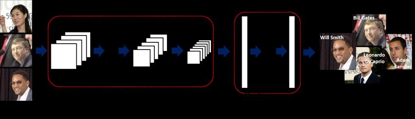
neural network (CNN, see Figure 1) have been introduced in face recognition, most notably
DeepFace [1], DeepID [2], FaceNet [3], and the VGG model [4]. These models apply convolution
and pooling repeatedly to extract local and global features of input image. In order to enhance
the classification ability, a set of fully connected layers are applied to feature maps from the
final convolutional layer. In a typical CNN, n feature maps are extracted from the input image
using n trained convolutional filters which are then transferred to the next layer. The size of the
extracted feature maps is reduced through a pooling layer, and m feature maps (derived from m
trained convolutional filters) are generated from the initially-obtained n feature maps through the
current convolutional layer. Typically, the number of feature maps outputted by the shallower-side
convolutional layers are limited by available memory and computational power, inevitably using
only a subset of useful patterns for face recognition. This can also be interpreted as excluding some
potentially useful patterns, which we define as untrained patterns in this paper, thereby yielding
suboptimal matching performance. Devising a way to reintroduce these untrained patterns into the
model is the main motivation of this work.
Appl. Sci. 2018, 8, 1561; doi:10.3390/app8091561 www.mdpi.com/journal/applsci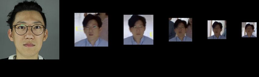
Appl. Sci. 2018, 8, 1561                                                                             2 of 12

                           Figure 1. An overview of a generic CNN architecture.

     In surveillance applications, face recognition methods can be applied to identify a target person.
Typically, images involved in these applications are acquired in an unconstrained environment with
potentially large variations in pose, illumination, expression, resolution and image quality. Recent face
recognition methods have achieved robustness to variations in pose, illumination, and expression,
but issues caused by low image resolution and quality still persist, requiring an expensive data
augmentation step to achieve advertised performance.
     In this paper, we propose PSI-CNN, a pyramid-based scale-invariant convolutional neural
network model, which utilizes additionally extracted untrained patterns to maintain high matching
accuracy in unconstrained environments. Our contributions are as follows:

1.    We present a comprehensive review of the literature which builds foundation to this work.
2.    Our proposed PSI-CNN model utilizes additionally extracted feature maps from various image
      resolutions, achieving robustness to scale changes in input images, potentially enabling its
      application in unconstrained environments with variable z-distance values.
3.    We provide an extensive analysis of the recognition performance achieved by models employing
      the PSI-CNN architecture. This is achieved by not only utilizing a publicly available database
      but also creating our own dataset collected under unconstrained environmental conditions with
      variable facial-region size.

     The structure of this paper is organized as follows. After reviewing relevant literature in Section 2,
our proposed PSI-CNN model is illustrated in Section 3. Experimental results and discussions are
included in Section 4, followed by conclusions in Section 5.

2. Related Work
     With the growth of importance in security, biometrics encoding personal characteristics such as
face, iris and fingerprints are widely used for person identification. Among them, face recognition is
becoming more prevalent thanks to the recent deep learning-based methods steadily improving the
identification accuracy.
     Face recognition can be categorized into three groups: holistic-based, partial-based, and deep
learning-based approaches. Holistic-based approaches utilize global facial characteristics as features
for identification. Many traditional methods such as Eigenfaces [5] and Fisherfaces [6] (based on the
linear discriminant analysis (LDA)), could be classified as holistic-based approaches.
     Turk et al., introduced Eigenface [5], which is a face recognition method based on the principal
component analysis (PCA). This method approximates an image as a vector of principal components
by projecting into the subspace of eigenvectors, which are calculated from the covariance matrix
of the training data. In this work, the eigenvectors represent the axes which can express the
distribution of training data. By sorting and selecting eigenvectors according to their respective
eigenvalues, one can reduce the dimension of input image without losing too much information.
Belhumeur et al., proposed a Fisherface-based face recognition method, which has higher recognition
accuracy than that of Eigenface [6]. The method is based on the LDA and projects given images into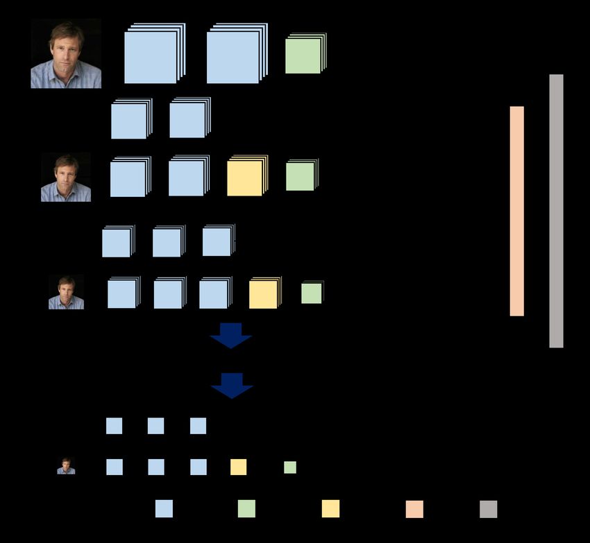
Appl. Sci. 2018, 8, 1561                                                                             3 of 12

Fisher’s linear discriminant vectors, which best explain the inter-class and intra-class relationships.
These two methods are the representative methods of the holistic-based approaches. Since
holistic-based approaches compute a vectorized matrix from the training dataset, these methods
are highly dependent to the characteristics of the training set used, and consequently they are sensitive
to environmental conditions such as illumination, pose and expression. Therefore, holistic-based
approaches require image normalization (e.g., through alignment of face region or normalization of
illumination) in order to improve the matching accuracy.
     Partial-based approaches were proposed to overcome the aforementioned weaknesses of the
holistic-based approaches. These approaches divide face region into grids and extract local facial
features. Well-known partial-based methods include the local binary patterns (LBP), scale-invariant
feature transform (SIFT) and histogram of gradients (HOG).
     Ahonen et al., proposed a face recognition method based on local binary patterns (LBP),
which analyze the patterns of the facial region [7]. This LBP method generates binary patterns
by comparing the value of the center pixel with that of its neighboring pixels in each local window.
Assuming that the size of the local window is 3 × 3 (i.e., nine pixels), the LBP operator represents each
pixel as 0 or 1 using a simple binary comparison. For instance, if a pixel value is greater than that
of the center pixel, then LBP outputs 1, otherwise it outputs 0. Also, the LBP-based face recognition
method transforms the extracted binary codes into uniform patterns. The uniform patterns consider
the number of transitions from 0 to 1 and the length of 1. From that, it can describe the texture of facial
skins which include edge and point information. Finally it represents these patterns as a histogram and
recognizes user by calculating the distance between the enrolled features and the features from input
image . The LBP-based method demonstrated then-high performance despite its relatively simple
architecture. Direct extensions of this work include local ternary patterns (LTP) and three-patch LBP
(TP-LBP) [8,9].
     After the success of the LBP method, several partial-based approaches were proposed and utilized.
In [10,11], the authors applied the SIFT and HOG algorithms respectively for partial feature-based
face recognition. Both methods have the advantage of being able to robustly extract facial features in
presence of local pose variations and illumination changes. Geng et al. introduced Volume-SIFT (VSIFT)
and Partial-Descriptor-SIFT (PDSIFT), which are extended versions of the original SIFT descriptor [10].
The SIFT algorithm is commonly used for object detection and recognition as its descriptor is invariant
to changes in scale and rotation. By applying SIFT to face recognition tasks, the authors were able to
extract robust facial features and compare the matching performance against other methods based on
holistic approaches. Deniz et al., applied HOG features for face recognition [11]; the authors detected
facial landmarks from input image, around which they set small areas of patches and extracted a HOG
descriptor from each patch. In this work, HOG features were extracted by applying patches of different
sizes, and combining these varying features were shown to improve the recognition performance.
     Chen et al. argued that high dimensionality leads to high performance, and demonstrated this
by comparing the proposed high-dimensional LBP method against the original method and other
then-state-of-the-art methods [12]. In this work, the authors initially detected 27 facial landmarks from
input image and created one 40 × 40-sized patch per landmark centered on the corresponding landmark
position. The designated patch region was divided into 4 × 4 non-overlapping cells, and facial features
were extracted from each divided cell by applying the LBP operator. In order to enhance scale
invariance, the authors resized the input image over five steps and performed the above procedure
repeatedly. From this, high-dimensional LBP features were generated by concatenating the extracted
feature vector from each cell, leading to a feature space dimension of around 100 K. The authors
applied PCA to reduce this dimension to a controllable size of 400. Experimental results showed that
the high-dimensional LBP features outperformed the low-dimensional LBP and other state-of-the-art
methods for the Labeled Faces in the Wild (LFW) dataset with unrestricted protocol [13]. Its matching
accuracy is 93.18%, which was the-state-of-the art accuracy. (The matching accuracy of the prior best
was about 90%).
Appl. Sci. 2018, 8, 1561 4 of 12
Since the success of deep learning in many areas of computer vision, several deep learning-based
methods have been proposed for face recognition. Overall, these methods attempt to extract feature
vectors encompassing both holistic and partial characteristics. Taigman et al. proposed a deep learning
framework for face recognition called “DeepFace”, which aligns input face image based on 3D face
model and extracts the corresponding feature vector from a nine-layer CNN [1]. The model was trained
by using approximately four million facial images acquired from around 4000 people. DeepFace adopts
an end-to-end metric learning model called the Siamese network, which directly predicts whether
the same person is observed in both of two input images. To enhance the recognition performance,
the authors combined several deep learning-based method, including the previously-mentioned
Siamese network. Subsequently, it achieved 97.37% of matching accuracy on the LFW dataset with
unrestricted protocol, which is very close to human recognition accuracy (≈ 97.5%).
After the introduction of DeepFace, many other deep learning-based methods have been proposed.
Sun et al.’s deep hidden identity features (DeepID) [2] detects five facial landmarks by using Sun et al.’s
method [14] and aligns input face by considering the centers of eyes and mouth. From the aligned face
image, the authors extracted feature vectors from 60 face patches, which are generated by considering
10 regions, three scales, and RGB or gray channels. They trained 60 convolutional networks (one
per face patch) where each network outputs two 160-dimensional feature vectors. Thus, the total
dimension of the concatenated feature vector is = 160 × 2 × 60 = 19,200. Finally, a joint Bayesian
method considering identity and intra-personal variation is applied to check if the same person is
observed in both of two input images [15].
Schroff et al. proposed a face recognition system called “FaceNet”, which directly extracts
a compact feature vector in the Euclidean space [3]. FaceNet generates a feature vector from input
image through a deep convolutional network (e.g., the Zeiler & Fergus network [16] and the Inception
network [17]) and embeds the feature vector into the Euclidean space by applying the triplet loss
method. For training the network based on the triplet loss, the authors utilized three images as
inputs, whereby two images are from the same identity and the other image is from a different person.
They defined one of two images of the same identity as anchor, and called the other image of the same
identity as positive and the image of a different identity as negative. Ideally, the Euclidean distance
between the anchor and the positive (d(ap) ) should be smaller than that between the anchor and the
negative (d(an) ). They minimized d(ap) − d(an) + α based on the equation d(ap) + α < d(an) , where α
is a margin variable to make larger gap between d(ap) and d(an) . The authors used about 200 million
images of eight million unique identities to train the network, achieving 99.63% recognition accuracy
on the LFW dataset with unrestricted, labeled outside the data protocol.
Parkhi et al. collected a large-scale face dataset called VGG-Face, and proposed the VGG
face model for face recognition [4]. The VGG-Face database contains about 2.6 millions images
of 2622 celebrities with manual filtering. The network architecture comprises five convolution blocks
and three fully connected layers connected in series. Each convolution block comprises of two or three
convolutional layers with max pooling to reduce the size of the output feature map. This network
was trained by using the VGG-Face database only, which is much smaller than the amount of training
data used by [1,3]. They demonstrated the efficiency of their database and network architecture
by achieving the recognition accuracy of over 97% on the LFW dataset with unrestricted protocol.
Applying the triplet loss from [3] further improves the accuracy by 1.8%.
A more concise review of the literature and classifications of the aforementioned face recognition
methods can be found in Table 1.Appl. Sci. 2018, 8, 1561 5 of 12
Table 1. A summary of past and current face recognition methods
Approaches Methods Characteristics
Generates Eigenfaces which represent the global
Eigenfaces (PCA) [5] characteristics of faces from training data by
extracting principal components.
Holistic-based
Computes representative axes which minimize
intra-class distances and maximizes inter-class
Fisherfaces (LDA) [6]
distances simultaneously from the global features
of the training data.
Describes the characteristics of local textures as
Local Binary Patterns [7] binary patterns by comparing the center pixel value
with that of its neighbors in each local window.
Applies the SIFT algorithm to extract local facial
SIFT [10]
Partial-based features which are scale and rotation-invariant.
Extracts local HOG feature from each divided grid
HoG Descriptor [11]
and concatenates all feature vectors.
Extracts 100K-dimensional LBP feature vector from
High-dimensional LBP [12]
multiple patches by considering scale variations.
Normalizes input face image based on a 3D
DeepFace [1] face model and extracts feature vectors by using
a 9-layer CNN.
Generates 60 patches from input image and extracts
a 160-dimensional feature vector from each patch.
DeepID [2]
Also, a joint-Bayesian method is applied to verify
whether the same person is observed or not.
Deep learning
Applies triplet loss to minimize distances between
images of the same identities and maximize
FaceNet [3]
distances between images of different identities.
Embeds each feature vector in the Euclidean space.
Consists of 13 convolutional layers and 3 fully
VGGFace [4] connected layers in series. Extracts feature vectors
by propagating through the network.
3. Proposed Framework
In this section, we first describe the main intuition behind our PSI-CNN architecture. Conventional
CNN models for face recognition comprise fewer number of filters in the shallower-side layers than
those in the deeper-end convolutional layers. For example, the VGG face model only uses 64 filters
in the first layer although the last convolutional layer utilizes 512 filters. The extracted feature map
is passed onto the next convolution step. As mentioned in Section 2, utilizing the characteristics of
local patterns can improve the recognition performance. However, since the sizes of input images
are typically over 200 × 200, the number of convolutional filters in the shallower layers are limited
by available memory and computation power. Consequently, some patterns are excluded from the
network despite these local characteristics being potentially useful for further enhancing the recognition
performance. Throughout this paper, we will refer to these excluded but potentially useful patterns as
untrained patterns.
As shown in Figure 2, PSI-CNN works by additionally extracting the aforementioned untrained
feature maps from a set of downsampled images (of the original input image) and fusing this
information during the convolution stages. We will use the schematic diagram of the PSI-CNN
architecture drawn in Figure 2 for further illustration of the model included in Section 3.1. (In this
diagram, (w, h, d) in Figure 2 refer to width, height, and number of feature maps respectively.)Appl. Sci. 2018, 8, 1561 6 of 12
Figure 2. An overview of our PSI-CNN architecture
3.1. PSI-CNN Model
PSI-CNN first passes input image through “Conv stage 1”, which comprises two ordinary
convolutional layers followed by a standard pooling layer. Each convolutional layer extracts d1
feature maps. Similar to the VGG face model, d1 is set to 64 and each feature map has size of 224 × 224.
After pooling, we yield 64 reduced feature maps of size 112 × 112.
Now, “Conv stage 2” is where the PSI-CNN model differs from other CNN-based approaches.
The 64 feature maps generated from “Conv stage 1” are passed through two additional convolutional
layers with 128 filters in “Conv stage 2”, generating d2 (= 128) feature maps in total. At the same time,
the factor-of-two-downsampled input image is used to generate d2 untrained feature maps of size
112 × 112. Thus, the total number of feature maps in “Conv stage 2” becomes 256 (=2 × 128).
If the above feature maps were to propagate directly to the next stage, the overall size of the
network would increase, consequently increasing the computational cost. To circumvent this issue,
we combine the feature maps resulted from “Conv stage 1” and the untrained feature maps from
the downsampled image by adopting a feature-level fusion process, maintaining a constant number
of feature maps. More specifically, each level of feature maps obtained by propagating through
the network is paired with its same-level untrained counterpart (i.e., feature maps derived from
image downsampling), and a combined feature map is generated by averaging each of these pairs.
By adopting this fusion procedure, it is possible to utilize a conventional CNN architecture without
modifying its foundational structure (e.g., number of feature maps and stride of convolution filters).
The subsequent stages are extended in the same way as in “Conv stage 2”.
After each convolution step, we apply the rectified linear unit (ReLU), which is an efficient
activation function that requires lower computation cost than other activations such as sigmoid or
hyperbolic tangent and avoids the problem of vanishing gradients during back-propagation [18].
Given a scalar input x, the ReLU function simply outputsAppl. Sci. 2018, 8, 1561 7 of 12
y = max(0, x ). (1)
After the last "Conv stage", 512 feature maps of size 7 × 7 are generated and converted to
a 1024-dimensional vector by applying a fully connected layer. Finally, a softmax layer is added
as a classifier. Note that this layer is only utilized at test time. The feature vector from the fully
connected layer is used to calculate the similarity between two images to identify whether they are
from the same person or not. To prevent over-fitting, we apply dropouts with 50% dropout probability
to edges between the fully connected layer and the classifier.
More details on the PSI-CNN architecture can be found in Table 2. Note that the PSI-CNN
framework is generic and may therefore be applied to other conventional convolutional networks
without modifying its basis structure.
Table 2. A detailed summary of the PSI-CNN structure
Stage Layer Name Number of Filters Size of Feature Map (H × W × D) Filter Size
Input layer 224 × 224 × 3 3×3
Conv1-1 64 224 × 224 × 64 3×3
Conv stage 1
Conv1-2 64 224 × 224 × 64 3×3
Pooling1 - 112 × 112 × 64 -
Conv2-1-1 128 112 × 112× 128 3×3
Conv2-1-2 128 112 × 112 × 128 3×3
ImageResizing2 - 112 × 112 × 3 -
Conv stage 2 Conv2-2-1 128 112 × 112 × 128 3× 3
Conv2-2-2 128 112 × 112 × 128 3×3
FeatureFusion2 - 112 × 112 × 128 -
Pooling2 - 56 × 56 × 256 -
Conv3-1-1 256 56 × 56 × 256 3×3
Conv3-1-2 256 56 × 56 × 256 3×3
Conv3-1-3 256 56 × 56 × 256 3×3
ImageResizing3 - 56 × 56 × 3 -
Conv stage 3 Conv3-2-1 256 56 × 56 × 256 3×3
Conv3-2-2 256 56 × 56 × 256 3×3
Conv3-2-3 256 56 × 56 × 256 3×3
FeatureFusion3 - 56 × 56 × 256 -
Pooling3 - 28 × 28 × 512 3×3
Conv4-1-1 512 28 × 28 × 512 3×3
Conv4-1-2 512 28 × 28 × 512 3×3
Conv4-1-3 512 28 × 28 × 512 3×3
ImageResizing4 - 28 × 28 × 3 -
Conv stage 4 Conv4-2-1 512 28 × 28 × 512 3×3
Conv4-2-2 512 28 × 28 × 512 3×3
Conv4-2-3 512 28 × 28 × 512 3×3
FeatureFusion4 - 28 × 28 × 512 -
Pooling4 - 14 × 14 × 512 -
Conv5-1-1 512 14 × 14 × 512 3×3
Conv5-1-2 512 124 × 14 × 512 3×3
Conv5-1-3 512 14 × 14 × 512 3×3
ImageResizing5 - 14 × 14 × 3 -
Conv stage 5 Conv5-2-1 512 14 × 14 × 512 3×3
Conv5-2-2 512 14 × 14 × 512 3×3
Conv5-2-3 512 14 × 14 × 512 3×3
FeatureFusion5 - 14 × 14 × 512 -
Pooling5 - 7 × 7 × 512 -
FC stage Fully connected - 1 × 1 × 1024 -Appl. Sci. 2018, 8, 1561 8 of 12
4. Experimental Results and Discussions
We evaluated the recognition performance of our proposed PSI-CNN model on two
datasets—Labeled Faces in the Wild (LFW) [13] and our custom dataset derived from CCTV cameras.
For this purpose, we used a 12GB NVIDIA TITAN X graphics card. For comparisons, we use a modified
version of the VGG face model as the baseline. This is because the original VGG model utilizes two fully
connected layers with each outputting 4096-dimensional vectors, meaning that the model requires large
amount of computation power and memory. To bypass this issue, we replaced the aforementioned fully
connected layers by a single smaller (1024-dimensional) fully connected layer. From our preliminary
empirical investigations, we were able to shrink the VGG model by almost 60% of its original size,
whilst maintaining 98.4% average matching accuracy on the above datasets. This implies that using
a fewer dimensional fully connected layer can be a computationally-efficient way of implementing
a high-performance face recognition method.
4.1. Model Training
For the purpose of training, we used the CASIA WebFace database, which comprises
approximately 500 K images of 10,575 different individuals collected from the Internet [19]. For the
baseline model, we optimized the 1024-dimensional fully connected layer via fine-tuning using the
CASIA WebFace database. After training the baseline model, we added “Conv stage 2”, which consists
of two convolutional layers that extract features from the factor-of-two-downsampled input image.
For the extended models, we set the learning rates for the existing layers and the newly added
convolutional layers to 0.0001 and 0.001 respectively, encouraging more versatile movements of the
newly added weights. The kernel size of each newly-trained convolutional filter was set to 3 × 3 in
order to maintain consistency with the reference VGG face model. All the model parameters were
optimized using the stochastic gradient descent (SGD) method with the weight decay factor set to
0.0005. Further “Conv stages” are added and optimized consecutively in a similar manner.
4.2. Performance Comparison on the LFW Dataset
The LFW database comprises 13,233 images of 5749 individuals taken in various environments.
It has become a de-facto evaluation benchmark dataset for face recognition. In this work, we evaluated
the performance under the unrestricted, labeled outside data protocol, which aims to measure how
many image pairs can be recognized correctly. It provides 6000 mixed pair of images, of which 3000 are
genuine pairs and others are imposters. These groups of pairs are further segregated into 10 subsets.
The matching performance is determined by the mean matching accuracy µ̂ and the standard deviation
of accuracies SE based on 10 cross validations. These are defined in (2) and (3) respectively, where pi
denotes the recognition rate of each test set. In this work, we computed the measurement of similarity
between each image pair based on their Euclidean distance.
∑10
i =1 p i
µ̂ = (2)
10
s
σ̂ ∑10
i =1 ( pi − µ̂ )
2
SE = √ , σ̂ = (3)
10 9
In order to extract feature vectors from input images, each image was resized to 256 × 256,
and total of 10 patches of size 224 × 224 were set on the original image and the flipped image (i.e.,
five patches per image). On each image, one patch was placed at the center of each image and the
other four were located near the image corners. We extracted feature vectors from these patches and
averaged them to generated the final feature vector.Appl. Sci. 2018, 8, 1561 9 of 12
For the first experiment, we compared the matching accuracy of each “Conv stage”-extended
model against the baseline. As shown in Figure 3 and Table 3, the performance is incrementally
enhanced by adding more convolutional stages. The proposed model with five convolutional stages
showed matching accuracy of 98.87%. Note that this score is achieved just by adopting the PSI-CNN
architecture and without incorporating additional learning framework such as triplet loss.
Table 3. Means and standard deviations of matching accuracies on the LFW dataset
Method Extended Conv. Stages µ̂ × 100(%) SE
Human - 97.53 -
Model 1 (baseline) - 98.40 0.0024
Model 2 Stage 2 98.60 0.0024
Model 3 Stage 2, 3 98.65 0.0020
Model 4 Stage 2, 3, 4 98.72 0.0018
Model 5 (Proposed model) Full Stage 98.87 0.0017
The experimental results demonstrate the effectiveness of untrained patterns in improving the
matching accuracy for face recognition.
Figure 3. The ROC curve of different models on the LFW dataset
4.3. Performance Comparison on Our CCTV Dataset
In the second experiment, we compared the performance of the baseline model and PSI-CNN
using our dataset generated from CCTVs. This dataset has around 1,500 images of 10 individuals,
comprising both high-quality images of frontal faces and low-resolution CCTV images for each person.
The number of genuine and imposter pairs are 2380 and 21,420 respectively. This CCTV dataset
was only used for the testing phase to demonstrate PSI-CNN’s robustness towards variations in
image resolutions and qualities. For performance comparisons, we used the equal error rate (EER),
which defines the error rate at which the false acceptance rate (FAR) and the false rejection rate (FRR)
are equal. FAR and FRR are calculated using (4) and (5) respectively. In these equations, true positive
(TP) and false negative (TN) refer to cases whereby the model identifies a true match as positive and
negative respectively, and vice versa for true negative (TN) and false positive(FP).
FP
FAR = × 100. (4)
TN + FPAppl. Sci. 2018, 8, 1561 10 of 12
FN
FRR = × 100. (5)
TP + FN
As shown in Table 4, the EER of the proposed model is 15.27%, which is 33% smaller than the
EER of the baseline model.
Additionally, we sampled and classified some CCTV images into groups (Probe 1 to probe 5)
according to their facial region size (see Figure 4 for a comprehensive example). In each group of
these sampled images, we compared the average matching distance achieved by the baseline and
PSI-CNN models. As shown in Figure 5, the proposed model achieves small error distance between
the reference frontal image and low-resolution CCTV images even when the resolution of the query
image is significantly reduced. This demonstrates PSI-CNN’s robustness to unfavorable changes in
image resolution and quality.
Figure 4. Some exemplary images in our CCTV dataset.
Figure 5. A performance comparison of face recognition models for different image resolutions based
on the Euclidean distance.
Table 4. A performance comparison between the baseline and PSI-CNN models on own CCTV dataset.
Method EER (%)
Baseline model 22.93
PSI-CNN model 15.27
4.4. Limitations
PSI-CNN was designed to utilize untrained patterns with the aim to resolve the weaknesses of the
current face recognition methods, which are sensitive to the resolution and quality of the input image.
However, this network still does not overcome problems arising from extreme pose variations and
occlusions largely due to lack of facial information. Developing a face recognition method robust to
facial occlusions (e.g., due to hair or accessories) and extreme pose variations is left for future work.Appl. Sci. 2018, 8, 1561 11 of 12
5. Conclusions
In this paper, we proposed PSI-CNN, a pyramid-based scale-invariant network for face
recognition. The proposed model additionally extracts untrained feature maps from downsampled
input image and fuses them with original feature maps, thereby encouraging the network to learn
potentially useful scale-independent information. Experimental results shows PSI-CNN outperforming
the baseline derived from the VGG face model in terms of matching accuracy. Furthermore, PSI-CNN
was able to maintain stable performance when tested on low-resolution images acquired from CCTV
cameras. These results demonstrate PSI-CNN’s robustness to changes in image resolution and quality.
Extending the proposed generic PSI-CNN architecture to solve other image-based problems would
also yield an interesting direction for future research.
Author Contributions: G.P.N. and I.-J.K. designed PSI-CNN architecture, H.C. and J.C. refined databases and
helped the experiments. All of the authors wrote and revised the paper.
Acknowledgments: This work was supported by the ICT R&D program of MSIT/IITP. [2017-0-00097,
Construction of Intelligence Information Industry Infrastructure] and [2017-0-00162, Development of Human-care
Robot Technology for Aging Society]. We thank Je Hyeong Hong at the Korea Institute of Science and Technology
for revising the paper.
Conflicts of Interest: The authors declare no conflict of interest.
References
1. Taigman, Y.; Yang, M.; Ranzato, M.; Wolf, L. DeepFace: Closing the Gap to Human-Level Performance in Face
Verification. In Proceedings of the IEEE Conference on Computer Vision and Pattern Recognition, Columbus,
OH, USA, 23–28 June 2014; pp. 1701–1708.
2. Sun, Y.; Wang, X.; Tang, X. Deep Learning Face Representation from Predicting 10,000 Classes. In Proceedings
of the IEEE Conference on Computer Vision and Pattern Recognition, Columbus, OH, USA, 23–28 June 2014;
pp. 1891–1898.
3. Schroff, F.; Kalenichenko, D.; Philbin, J. FaceNet: A Unified Embedding for Face Recognition and Clustering.
In Proceedings of the IEEE Conference on Computer Vision and Pattern Recognition, Boston, MA, USA,
7–12 June 2015; pp. 815–823.
4. Parkhi, O.M.; Vedaldi, A.; Zisserman, A. Deep Face Recognition. In Proceedings of the British Machine Vision
Conference, Swansea, UK, 7–10 September 2015.
5. Turk, M.; Pentland, A. Eigenfaces for Recognition. J. Cognit. Neurosci. 1991, 3, 71–86. [CrossRef] [PubMed]
6. Belhumeur, P.N.; Hespanha, J.P.; Kriegman, D.J. Eigenfaces vs. Fisherfaces: Recognition using Class Specific
Linear Projection. IEEE Trans. Pattern Anal. Mach. Intell. 1997, 19, 711–720. [CrossRef]
7. Ahonen, T.; Hadid, A.; Pietikainen, M. Face Description with Local Binary Patterns: Application to Face
Recognition. IEEE Trans. Pattern Anal. Mach. Intell. 2006, 28, 2037–2041. [CrossRef] [PubMed]
8. Tan, X.; Triggs, B. Enhanced Local Texture Feature Sets for Face Recognition under Difficult Lighting
Conditions. IEEE Trans. Image Process. 2010, 19, 1635–1650. [PubMed]
9. Wolf, L.; Hassner, T.; Taigman, Y. Effective Unconstrained Face Recognition by Combining Multiple
Descriptors And Learned Background Statistics. IEEE Trans. Pattern Anal. Mach. Intell. 2011, 33, 1978–1990.
[CrossRef] [PubMed]
10. Geng, C.; Jiang. X. Face Recognition Using SIFT Features. In Proceedings of the IEEE International Conference
on Image Processing (ICIP), Cairo, Egypt, 7–10 November 2009.
11. Deniz, O.; Bueno, G.; Salido, J.; De la Torre, F. Face Recognition Using Histograms of Oriented Gradients.
Pattern Reocgnit. Lett. 2011, 32, 1598–1603. [CrossRef]
12. Chen, D.; Cao, X.; Wen, F.; Sun, J. Blessing of Dimensionality: High-dimensional Feature and Its Efficient
Compression for Face Verification. In Proceedings of the IEEE Conference on Computer Vision and Pattern
Recognition, Portland, OR, USA, 23–28 June 2013; pp. 3026–3032.
13. Huang, G.B.; Mattar, M.; Berg, T.; Learned-Miller, E. Labeled Faces in the Wild: A Database for Studying Face
Recognition in Unconstrained Environments. In Proceedings of the Workshop on Faces in ’Real-Life’ Images:
Detection, Alignment, and Recognition, Marseille, France, 17–20 October 2008; pp. 7–49.Appl. Sci. 2018, 8, 1561 12 of 12
14. Sun, Y.; Wang, X.; Tang, X. Deep Convolutional Network Cascade for Facial Point Detection. In Proceedings
of the IEEE Conference on Computer Vision and Pattern Recognition, Portland, OR, USA, 23–28 June 2013;
pp. 3476–3483.
15. Chen, D.; Cao, X.; Wang, L.; Wen, F.; Sun, J. Bayesian Face Revisited: A Joint Formulation. In Proceedings of
the 12th European Conference on Computer Vision, Florence, Italy, 7–13 October 2012; pp. 566–579.
16. Zeiler, M. D.; Fergus, R. Visualizing and Understanding Convolutional Networks. In Proceedings of the 13th
European Conference on Computer Vision, Zurich, Switzerland, 6–12 September 2014; pp. 818–833.
17. Szegedy, C.; Liu, W.; Jia, Y.; Sermanet, P.; Reed, S.; Anguelov, D.; Erhan, D.; Vanhoucke, V.; Rabinovich, A.
Going Deeper with Convolutions. In Proceedings of the IEEE Conference on Computer Vision and Pattern
Recognition, Boston, MA, USA, 7–12 June 2015; pp.1–9.
18. Glorot, X.; Bordes, A.; Bengio, Y. Deep sparse rectifier networks. In Proceedings of the Fourteenth International
Conference on Artificial Intelligence and Statistics, Ft. Lauderdale, FL, USA, 11–13 April 2011; pp. 315–323.
19. Yi, D.; Lei, Z.; Liao, S.; Li, S.Z. Learning Face Representation from Scratch. arXiv 2014, arXiv:1411.7923.
c 2018 by the authors. Licensee MDPI, Basel, Switzerland. This article is an open access
article distributed under the terms and conditions of the Creative Commons Attribution
(CC BY) license (http://creativecommons.org/licenses/by/4.0/).You can also read