Predictive Community Computational Tools for Virtual Plasma Science Experiments
←
→
Page content transcription
If your browser does not render page correctly, please read the page content below
Predictive Community Computational Tools
  for Virtual Plasma Science Experiments

   J.-L. Vay, E. Esarey, S. Bulanov, A. Koniges
      Lawrence Berkeley National Laboratory
       J. Barnard, A. Friedman, D. Grote
      Lawrence Livermore National Laboratory

 Frontiers of Plasma Science Workshops - Town Hall

                 June 30-July 1, 2015

            Office of UNIVERSITY OF
                                                     1
            Science CALIFORNIA 1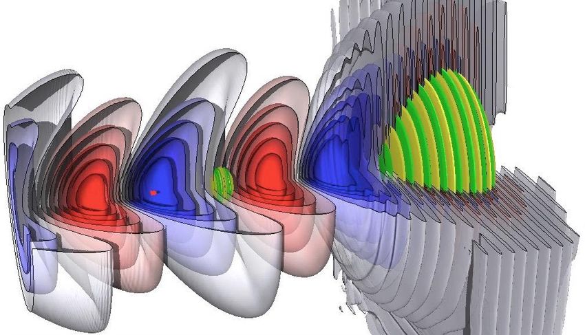
Advanced simulations play an increasingly important role in
            the exploration of new concepts.
                    Large scale 3-D simulations with Warp
      validated a new concept of injection of ultra-low emittance beam
                         in laser-plasma accelerator
                                                                             Two-color injection*.
                    Low
                    emittance
                    injected beam

                                                                      Pump laser            Plasma
                                                               Wake   pulse

                                                 Injection
                                                 laser pulse                   Simulations: Warp
                                                                               Visualization: VisIt

*L.-L. Yu, et al, Phys. Rev. Lett. 112, 125001 (2014)
                                     Office of UNIVERSITY OF
                                                                                                      2
                                     Science CALIFORNIA 2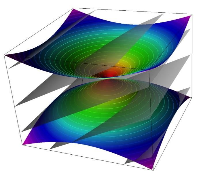
Advanced simulations play an increasingly important role in
    the design, operation and analysis of experiments.
                  Large scale simulations with INF&RNO*
          supported world record BELLA 4.25 GeV beam over 9 cm**
                        Laser optical spectra after 9 cm plasma (Ulaser=7.5 J)

                                                                        simulated spectra corrected for
                                                                        the instrument spectral response

*2015 NERSC HPC award                                  **W. P. Leemans, et al., Phys. Rev. Lett. 113, 245002 (2014)
                             Office of UNIVERSITY OF
                                                                                                                3
                             Science CALIFORNIA 3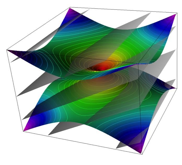
Large scale simulations (still) take too long!
Real machines need fast turnaround for real-time tuning.
Now
      2D-RZ simulations of BELLA                      3D simulation of novel injection scheme

                                                                                              Warp+VisIt

                         INF&RNO

 0.5 M CPU-HRS (~1 week for 9 cm plasma)               0.25 M CPU-HRS (~1.5 day for 1 mm plasma)

        Geometry            R, Z-CT              Geometry               X, Z-CT               3-D X, Y, Z-CT
       # grid cells      1,400x14,000           # grid cells          1,200x3,300            600x600x1,650
      # grid cells/kp       15x200             # grid cells/kp          65x140                 32x32x70
          Lplasma           ~9 cm                  Lplasma                           ~1 mm
      # time steps        12,000,000            # time steps           300,000                  150,000
         # cores             3,400                # cores               1,200                    6,144
        Runtime            150 hours             Runtime                1 hours                 36 hours
           Cost          0.5 M CPU-HRs                Cost           1.2 k CPU-HRs           0.22 M CPU-HRs

                            Office of UNIVERSITY OF
                                                                                                               4
                            Science CALIFORNIA 4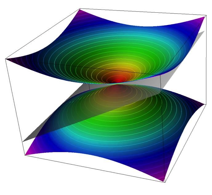
Future computational needs are extremely high
Laser plasma acceleration
• 3-D BELLA simulation: ~ 500 M CPU-HRs
• 3-D k-BELLA simulation: ~ 50 M CPU-HRs
• Parametric studies: × 100
10-100 Billions of CPU-HRs
Ion acceleration (BELLA-i)
• Dx≈l/103 to resolve l solid density plasma
small box of (10l)3 results in ≈1012 cells
• Time scales: from fs (PIC) to ns (MHD)
100M to Billions of CPU-HRs/run
Others also stressing computational needs
High-intensity Self-organization
Flying plasma mirrors Laser-driven X-ray sources laser-matter interactions in ExB discharges
Office of UNIVERSITY OF
5
Science CALIFORNIA 5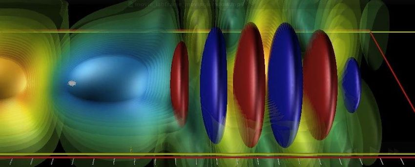
Confluence of exascale computers & novel algorithms
to deliver better, bigger & faster computing
Goal is multi-scale multi-physics:
Combine modules/codes
(MHD+PIC+target physics+…)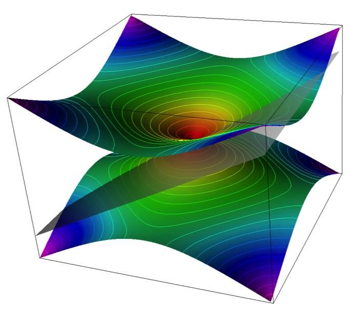
Task is complex & calls for cross-discipline teams
Need for tight coupling, as
process not unidirectional:                                                Examples
                                               Lorentz boosted frame Parallel spectral solver

              Physics

         Equations       Codes

               Science
   Applied       Algo-    Computer
                                                Uses special relativity to        Uses finite speed of light
    Math        rithms     Science              speedup simulations by            to enable direct scaling
                                                orders of magnitude.              to many cores.
                                                J.-L. Vay, Phys. Rev. Lett. 98,   J.-L. Vay, I. Haber & B. B.
                                                130405 (2007)                     Godfrey, J. Comput. Phys. 243,
 w/ physics used to alter                                                         260-268 (2013)
 algorithms & codes.

         Algorithmic developments can lead to very high payoffs
                                 Office of UNIVERSITY OF
                                                                                                                   7
                                 Science CALIFORNIA 7
Laser plasma acceleration (LPA) analogy

surfer      wake                    boat

e- beam     wake                    laser
          Office of UNIVERSITY OF
                                            8
          Science CALIFORNIA 8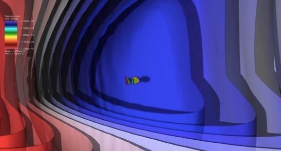
Modeling from first principle is very challenging
For a 10 GeV scale stage:
~1mm wavelength laser propagates into ~1m plasma
millions of time steps needed
(similar to modeling 5m boat crossing ~5000 km Atlantic Ocean)
Office of UNIVERSITY OF
9
Science CALIFORNIA 9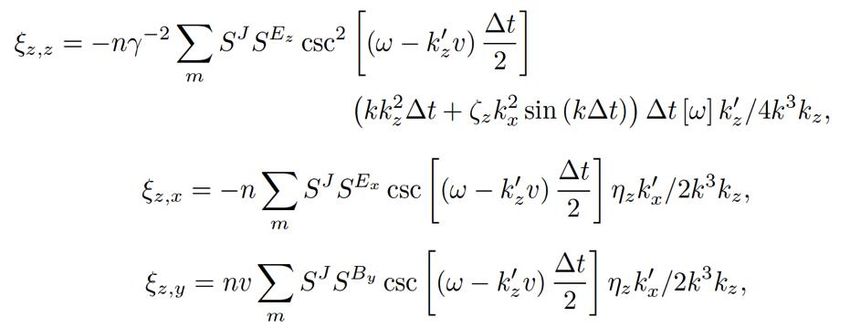
Solution: model in frame moving near the speed of light*
Lab frame Boosted frame = 100
l≈1. mm l’=200. mm
Hendrik Lorentz
L≈1. m L’=0.01 m
compaction
1. m/1. mm=1,000,000 0.01 m/200. mm=50. X20,000
• BELLA-scale w/ ~ 5k CPU-Hrs: 2006 - 1D run 2011: 3D run
• Progress in envelope solvers (Benedetti) can be combined for
further speedups
*J.-L. Vay, Phys. Rev. Lett. 98, 130405 (2007)
Office of UNIVERSITY OF
10
Science CALIFORNIA 10Relativistic plasmas PIC subject to “numerical Cherenkov”
Numerical dispersion leads to crossing of EM field and plasma modes -> instability.
Exact Maxwell Standard PIC
*B. B. Godfrey, “Numerical Cherenkov instabilities in electromagnetic particle codes”, J. Comput. Phys. 15 (1974)
Office of UNIVERSITY OF
11
Science CALIFORNIA 11Space/time discretization aliases more crossings in 2/3-D
Exact Maxwell Standard PIC
light light
w w
kx kx
plasma kz plasma kz
at at
b=0.99 b=0.99
Need to consider at least first aliases mx={-3…+3} to study stability.
Office of UNIVERSITY OF
12
Science CALIFORNIA 12Space/time discretization aliases more crossings in 2/3-D
Exact Maxwell Standard PIC
aliases aliases
light light
w w
kx kx
plasma kz plasma kz
at at
b=0.99 b=0.99
Need toAnalysis
considercalls for full
at least firstPIC numerical
aliases dispersion
mx={-3…+3} relation
to study stability.
Office of UNIVERSITY OF
13
Science CALIFORNIA 13Numerical dispersion relation of full-PIC algorithm*
2-D relation
(Fourier
space):
*B. B. Godfrey, J. L. Vay, I. Haber, J. Comp. Phys. 248 (2013)
Office of UNIVERSITY OF
14
Science CALIFORNIA 14Numerical dispersion relation of full-PIC algorithm (II)
*B. B. Godfrey, J. L. Vay, I. Haber, J. Comp. Phys. 248 (2013)
Office of UNIVERSITY OF
15
Science CALIFORNIA 15Numerical dispersion relation of full-PIC algorithm (III)
Then simplify and solve with Mathematica…
Office of UNIVERSITY OF
16
Science CALIFORNIA 16Tremendous progress on analysis/mitigation of NC
in recent years
• Analysis of Numerical Cherenkov has been generalized:
• to finite-difference PIC codes (“Magical” time step explained):
• B. B. Godfrey and J.-L. Vay, J. Comp. Phys. 248 (2013) 33.
• X. Xu, et. al., Comp. Phys. Comm., 184 (2013) 2503.
• to pseudo-spectral PIC codes:
• B. B. Godfrey, J. -L. Vay, I. Haber, J. Comp. Phys., 258 (2014) 689.
• P. Yu et. al, J. Comp. Phys. 266 (2014) 124.
• Suppression techniques were developed:
• for finite-difference PIC codes:
• B. B. Godfrey and J.-L. Vay, J. Comp. Phys. 267 (2014) 1.
• B. B. Godfrey and J.-L. Vay, Comp. Phys. Comm., in press
• for pseudo-spectral PIC codes:
• B. B. Godfrey, J.-L. Vay, I. Haber, IEEE Trans. Plas. Sci. 42 (2014) 1339.
• P. Yu, et. al., arXiv:1407.0272 (2014)
Applications to relativistic laboratory and space plasmas.
Office of UNIVERSITY OF
17
Science CALIFORNIA 17A more coordinated program would boost the
development of the next generation of simulations tools
Computational toolkits can rival (or surpass) the complexity of experiments
• needs to reproduce the complexity of experimental setups,
• discretization -and other numerical artifacts- add layer of complexity
that needs to be fully understood and controlled.
A coordinated, community program would be most effective:
• develop & maintain integrated comprehensive kit is an enormous task:
• collection of exascale-ready (PIC, MHD, fluid, radiation, QED, MD, EOS, etc.) modules,
• current situation is suboptimal: many codes within projects without coordination,
• very few codes are open source: inhibits co-development, verifiability and adoption.
Can benefit from links with/experience from other communities:
• SciDAC programs
• DOE-HEP Forum for Computational Excellence (HEP-FCE): coordinates across HEP
• Consortium for Advanced Modeling of Particle Accelerators (CAMPA)
• coordinates code development between LBNL, SLAC and FNAL
• Astrophysics: e.g. FLASH
Office of UNIVERSITY OF
18
Science CALIFORNIA 18Conclusion
Plasma physics involves tightly coupled non-linear multi-scale/physics phenomena
• large-scale modeling, w/ theory/experiment, is key to understanding of complexity
Computational plasma physics is a very active field; better computational tools
accelerate discoveries across plasma science
• computational methods/codes are very general
• benefits to society over a wide range of applications
• medical technology (e.g. ion-driven cancer therapy, light sources for bioimaging),
• energy (e.g. fusion sciences),
• basic physics (e.g. HEDLP science, space plasmas science, charged particle traps),
• accelerators (e.g. HEP and rare isotope facilities),
• industry (e.g. plasma processing),
• national security (e.g. science-based stockpile stewardship, gamma sources).
Exascale computing is key to enabling “real-time” virtual experiments
• but not silver bullet: significant investments are needed in algorithms/codes
A coordinated, community effort will be most effective
• cross-institutional development of integrated comprehensive kit to maximize resources
Office of UNIVERSITY OF
19
Science CALIFORNIA 19Extras
Office of UNIVERSITY OF
20
Science CALIFORNIA 20Warp: PIC framework for modeling of beams, plasmas & accel.
http://blast.lbl.gov/BLASTcodes_Warp.html; http://warp.lbl.gov
• Geometry: 3-D (x,y,z) axisym. (r,z) 2-D (x,z) 2-D (x,y)
x
y z
• Reference frame: lab moving-window Lorentz boosted
z z-vt (z-vt); (t-vz/c2)
• Field solvers
- electrostatic/magnetostatic - FFT, multigrid; AMR; implicit; cut-cell boundaries
R (m)
Versatile conductor generator Automatic meshing
accommodates complicated around ion beam
structures source emitter
Z (m)
- Fully electromagnetic – Yee/node centered mesh, arbitrary order, spectral, PML, MR
• Accelerator lattice: general; non-paraxial; can read MAD files
- solenoids, dipoles, quads, sextupoles, linear maps, arbitrary fields, acceleration.
• Particle emission & collisions
- particle emission: space charge limited, thermionic, hybrid, arbitrary,
- secondary e- emission (Posinst), ion-impact electron emission (Txphysics) & gas emission,
- Monte Carlo collisions: ionization, capture, charge exchange.
Office of UNIVERSITY OF
21
Science CALIFORNIA 21Warp is parallel, combining modern and efficient programming languages
• Parallellization: MPI (1, 2 and 3D domain decomposition)
Parallel strong scaling of Warp
3D PIC-EM solver on Hopper
supercomputer (NERSC)
• Python and FORTRAN*: “steerable,” input decks are programs
From warp import * Imports Warp modules and routines in memory
…
nx = ny = nz = 32 Sets # of grid cells
dt = 0.5*dz/vbeam Sets time step
…
initialize() Initializes internal FORTRAN arrays
step(zmax/(dt*vbeam)) Pushes particles for N time steps with FORTRAN routines
…
*http://hifweb.lbl.gov/Forthon – dpgrote@lbl.gov
Office of UNIVERSITY OF
22
Science CALIFORNIA 2222Sample applications
Space charge dominated beams Beam dynamics in rings Multi-charge state beams
Injection
Transport
Neutralization
UMER LEBT – Project X
22
Vy vs Y
Traps Electron cloud effects 1.0
Multi-pacting
10^+7
0.5
Vy
0.0
-0.5
Warp Courtesy H. Sugimoto
Warp-Posinst
Alpha anti-H trap Paul trap SPS “Ping-Pong”
-1.0 effect 0.001
0.000 0.002 0.003
Y
z window0 = -2.2400e-02, 2.2400e-02
Laser plasma acceleration 3D Coherent Synchrotron Radiation Free Electron Lasers
Step 240, T = 1.1628e-9 s, Zbeam = 0.0000e+0 m
Rectangular Waveguide: BDC=0; E=34.22kV/m
dt= 4.8ps;nx,ny,nz=64x8x128;egrdnx,ny,nz=22x16x44
R.A. Kishek warp r2 rect!_MPC!_noB!_01
Office of UNIVERSITY OF
23
Science CALIFORNIA 23You can also read