R 1317 - Declining natural interest rate in the US: the pension system matters by Jacopo Bonchi and Giacomo Caracciolo - Banca d'Italia
←
→
Page content transcription
If your browser does not render page correctly, please read the page content below
Temi di discussione
                (Working Papers)

                Declining natural interest rate in the US:
                the pension system matters

                by Jacopo Bonchi and Giacomo Caracciolo
February 2021

                                                                      1317
                                                             Number
Temi di discussione (Working Papers) Declining natural interest rate in the US: the pension system matters by Jacopo Bonchi and Giacomo Caracciolo Number 1317 - February 2021
The papers published in the Temi di discussione series describe preliminary results and
are made available to the public to encourage discussion and elicit comments.
The views expressed in the articles are those of the authors and do not involve the
responsibility of the Bank.

Editorial Board: Federico Cingano, Marianna Riggi, Monica Andini, Audinga
Baltrunaite, Marco Bottone, Davide Delle Monache, Sara Formai, Francesco
Franceschi, Adriana Grasso, Salvatore Lo Bello, Juho Taneli Makinen, Luca
Metelli, Marco Savegnago.
Editorial Assistants: Alessandra Giammarco, Roberto Marano.

ISSN 1594-7939 (print)
ISSN 2281-3950 (online)
Printed by the Printing and Publishing Division of the Bank of Italy
DECLINING NATURAL INTEREST RATE IN THE US:
                           THE PENSION SYSTEM MATTERS

                            by Jacopo Bonchi* and Giacomo Caracciolo†

                                                  Abstract

        The natural interest rate is the level of the real interest rate compatible with potential
output and stable prices. We develop a life-cycle model and calibrate it to the US economy to
quantify the role of the public pension scheme for the past and future evolution of the natural
interest rate. Between 1970 and 2015, the pension reforms mitigated overall the secular
decline in the natural interest rate, raising it by around one percentage point and thus
counteracting the downward pressure from adverse demographic and productivity patterns. As
regards the future, we simulate the effects of the demographic trends expected between 2015
and 2060, combined with alternative pension reforms and productivity growth scenarios. We
rank the different policy options according to a welfare criterion and study the implications
for the natural interest rate. In terms of welfare, a reduction in the replacement rate
outperforms an increase in the contribution rate under the “normal growth” scenario but the
opposite is true under the “stagnant growth” scenario.

JEL Classification: E60, H55.
Keywords: natural interest rate, pensions, population ageing, secular stagnation, demography,
social security.
DOI: 10.32057/0.TD.2021.1317

_______________________________________
* LUISS, e-mail: jbonchi@luiss.it
† Bank of Italy, e-mail: giacomo.caracciolo@bancaditalia.it
8
Contents
1. Introduction ........................................................................................................................... 5
2. Theoretical model ................................................................................................................ 10
2.1 Setup ............................................................................................................................. 10
2.2 Demographics, pension reforms and the natural interest rate ...................................... 13
2.2.1 Reform of the replacement rate ........................................................................... 14
2.2.2 Reform of the contribution .................................................................................. 15
2.2.3 Reform of the retirement age ............................................................................... 15
3. Quantitative model .............................................................................................................. 17
3.1 Households ................................................................................................................... 17
3.2 Firms ............................................................................................................................. 19
3.3 Government .................................................................................................................. 19
3.4 Pension system ............................................................................................................. 20
4. The natural interest rate in the past ...................................................................................... 23
4.1 Results .......................................................................................................................... 26
5. The natural interest rate in the future................................................................................... 28
5.1 Calibration .................................................................................................................... 30
5.2 Results .......................................................................................................................... 30
5.2.1 Stationary equilibrium and transition dynamics .................................................. 30
5.2.2 Welfare analysis .................................................................................................. 33
6. Conclusions .......................................................................................................................... 34
References ................................................................................................................................ 37
Appendices ............................................................................................................................... 43
A. Quantitative model ....................................................................................................... 43
A.1 Households ............................................................................................................ 43
A.2 Firms ...................................................................................................................... 44
A.3 The pension benefit formula according to the OASDI program ........................... 46
A.4 Competitive stationary equilibrium ....................................................................... 49
A.5 Solution method..................................................................................................... 49
A.6 The age profile of labor productivity..................................................................... 51
B. The natural interest rate in the past............................................................................... 51
B.1 Alternative calibration of the retirement age ......................................................... 51
C. The natural interest rate in the future ........................................................................... 53
C.1 Calibration ............................................................................................................. 53
C.2 Endogenous debt-to-GDP ratio .............................................................................. 541 Introduction
Based on the evidence of a sluggish recovery, a low inflation rate and policy rates at
the zero lower bound, the idea of a “secular stagnation”, formulated by Hansen (1939),
has recently gained new momentum. The new theory of secular stagnation explains the
declining trend in the US natural interest rate as the result of a widening gap between
saving and investment and it puts forward several candidates as potential drivers of
such phenomenon (Summers, 2014). The list of candidates includes, to name a few,
population ageing, productivity slowdown, rising income inequality and the decline in
investment goods prices. Among these, demographics and productivity stand out as
the most quantitatively relevant (Gagnon et al., 2016; Eggertsson et al., 2019). The
idea of a “natural” level of the real interest rate, the so-called r∗ , consistent with the
potential output and stable prices, is central to monetary policy. When the natural
interest rate stabilizes at very low or even negative levels, as suggested by the recent
estimates for the US economy (Laubach and Williams, 2016; Negro et al., 2017), the
margins to cut the policy rate are greatly reduced, and the central bank could hit the
zero lower bound (ZLB) more frequently. As more frequent ZLB episodes would imply
deeper and prolonged recessions (Kiley and Roberts, 2017), it is crucial to understand
the driving forces of the natural interest rate and whether their effect is going to vanish
or persist in the future.
Despite the extensive analysis of many possible secular stagnation determinants,
the existing literature has disregarded an economic institution that crucially affects
the saving behavior: the pension system and its rules. This paper investigates the
quantitative importance of the public pension system for the US natural interest rate
in the last fifty years, and it carries out a prospective analysis of its future impact, in
response to population ageing, under different policy and productivity growth scenarios.
The omission of Social Security and its evolution over time in the literature on the
drivers of the natural interest rate is notable for, at least, two reasons.
First, the size of the US public pension system, officially the Old-Age, Survivors,
and Disability Insurance (OASDI) program, is not negligible, implying a potentially
relevant impact on saving and the natural interest rate.1 Figure 1 depicts US public
1
The OASDI program operates under a pay-as-you-go (PAYG) basis providing benefits to retirees and
disabled people. The current workers finance the benefits of the current retirees through payroll taxes,
and the pension system keeps the financial resources in two trust funds, the Old-Age and Survivors
Insurance Trust Fund (OASI) for retirement and the Disability Insurance Trust Fund (DI) for disability,
which pay out effectively the benefits.
5Figure 1: Public pension spending in the OECD countries
Source: OECD
18
Australia
Canada
France
16
Germany
Public pension spending as % of GDP
Italy
OECD
14 UK
USA
12
10
8
6
4
2
1980 1985 1990 1995 2000 2005 2010 2015
Year
pension spending in terms of GDP, along with that of some OECD countries.
Second, the dimension of the US public pension system is expected to vary sig-
nificantly in the future.The demographic transition towards an older society is at an
earlier stage in the US than in other advanced countries, due to a delayed increase in life
expectancy and a more muted decline in the fertility rate (Figure 2). As a consequence,
the old-age dependency ratio (DR) has been more stable, mitigating the pressure on
the budget of the pension system. However, the DR between people aged 65 and over
and those aged 20-64 is expected to increase in the future, forcing the US government
to speed up the reform process.23 Indeed, a higher DR threatens the financial sustain-
ability of the public PAYG schemes, because an ever-smaller working population would
finance the pension benefits of more retirees.
2
Most of the advanced countries have already implemented pension reforms to contain expenditure
and increase revenues, mainly through changes in the replacement rate, the retirement age and the
contribution rate (OECD, 2017). Although the US has put in place some minor reforms, the major
pension reform, the so-called “Simpson-Bowles” plan, was never adopted (OECD, 2013).
3
The US DR did not increase markedly between 1975 and 2015 (from 19.7% to 24.6%), but it will rise
to 40.3% over the period 2015-2050 (OECD, 2017). Consequently, the OASI will exhaust in 2034 (2019
Annual Report of the Board of Trustees of the OASI and DI), and the deterioration in the funding
position of the OASI will presumably call for substantial pension reforms.
6Figure 2: Demographic trends
Source: World Bank
82 3
EU EU
OECD OECD
US 2.8 US
80
2.6
78
Life expectancy at birth
Total fertility rate
2.4
76
2.2
74
2
72
1.8
70
1.6
68 1.4
1970 1980 1990 2000 2010 1970 1980 1990 2000 2010
We aim to identify and measure the quantitative impact of the public pension
system and its reforms on the natural interest rate, in the past and the future. To that
aim, we first develop an overlapping generations (OLG) model with three generations
for illustrative purposes. Although highly stylized, the model explains the relationship
between a PAYG pension scheme and the natural interest rate. Furthermore, it clari-
fies the interaction between demographic changes and pension reforms, providing clear
theoretical insights to understand the quantitative impact of the pension system on the
natural interest rate under different demographic and technological conditions. As a
result, the toy model shows that, following the same demographic shock, some types of
pension system adjustments mitigate the direct effect of the shock on the equilibrium
interest rate, while some others amplify it.
We then employ a more realistic quantitative life-cycle model, which is calibrated
to the US economy. Specifically, we run two quantitative exercises. Firstly, we decom-
pose the decline in the natural interest rate between 1970 and 2015 and we examine the
role of the pension system and its reforms. On the one hand, simply accounting for the
pension system, even without considering its changes over time, mitigates the impact of
the forces putting downward pressure on the natural interest rate. On the other hand,
7the adjustments in the US pension system have prevented the natural interest rate from
dropping further by around 1%, counteracting the negative effect of demographic and
technological trends. The last result is due to the past evolution of the US pension
scheme, which has become more generous in terms of replacement rate in the last fifty
years.
Secondly, we simulate the demographic changes predicted by the United Nations
for the US population between 2015 and 2060 and we study the expected evolution of
the natural interest rate implied by alternative pension reforms along the transition.
Our analysis focuses deliberately on the case in which the real interest rate is lower
than the economy’s growth rate g, due to a falling r∗ . While demographic trends are
slow-moving and thus easily predictable, the evolution of productivity is an object of
speculation. Consequently, we compare two different scenarios: one, named “stagnant
growth”, in which the rate of productivity growth remains at the 2015 low level until
2060, and another one of “normal growth” in which productivity grows at 2% per year.
Our results indicate that the future natural interest rate is subject to high vari-
ability depending on the scenario-reform combination, with its long run value ranging
between +45 to -160 basis points relative to the starting point in 2015. In particu-
lar, it always decreases with “stagnant growth”, while it always increases with “normal
growth”, for a given public debt-to-GDP ratio. More importantly, the ranking among
the different pension adjustments, based on a welfare criterion, depends on the evolu-
tion of productivity, and it is driven by the implied effect on the natural interest rate,
r∗ . In particular, a reduction in the replacement rate outperforms, in terms of welfare,
an increase in the contribution rate in the “normal growth” scenario and vice versa in
the “stagnant growth” case. This result goes hand-in-hand with the fact that the reform
of the replacement rate mitigates the fall in r∗ as much as the reform of the contribution
rate with “normal growth”, but it greatly amplifies the fall in r∗ with “stagnant growth”.
Related literature
Our contribution lies in the intersection between two strands of the economic litera-
ture. The first one concerns secular stagnation and the historical decline in the natural
interest rate (Ikeda and Saito, 2014; Summers, 2014; Gordon, 2015; Carvalho et al.,
2016; Gagnon et al., 2016; Kara and von Thadden, 2016; Cooley and Henriksen, 2018;
Barany et al., 2018; Eggertsson et al., 2019; Rachel and Summers, 2019; Auclert et
8al., 2020; Bielecki et al., 2020; Papetti, 2020). The second one, less recent, regards the
effects of PAYG pension system reforms (de Nardi et al., 1999; Börsch-Supan et al.,
2006; Krueger and Kubler, 2006; Attanasio et al., 2007; Krueger and Ludwig, 2007).
The empirical phenomena that motivate, and so connect, the two are population age-
ing and the evolution of technology over time. We contribute to the literature on the
drivers of the historical decline in r∗ by studying the implications of the pension reforms
implemented in the US in response to demographic trends experienced in the past and
expected in the future. Our analysis distinguishes itself from the second strand as we
investigate PAYG reforms in a secular stagnation environment featuring r < g. By
focusing on a dynamically inefficient economy, our work emphasizes how the implicit
return of the PAYG asset, which is larger than the real interest rate, influences the
desirability of different pension adjustments forced by demographic changes. Although
r < g has often been regarded as a purely theoretical case (Abel et al., 1989), the recent
evidence by Geerolf (2018) and Blanchard (2019) proves that it is a real possibility for
the advanced economies, including the US, especially if the declining trend in r∗ will
persist in the future.
Our work is very close to Attanasio et al. (2007) and Krueger and Ludwig (2007),
who study the impact of alternative pension reforms, aimed at restoring the sustain-
ability of the PAYG system in response to demographic trends, on prices and welfare.
We depart from their approach as we examine a closed, dynamically inefficient, econ-
omy. Carvalho et al. (2016) and Kara and von Thadden (2016) adopt a “perpetual
youth” model à la Gertler (1999), in which the probability of dying is not age-specific,
to study the effect of pensions and demographics on interest rates. By employing this
framework, Carvalho et al. (2016) show that the pension system and its reforms did
not counteract significantly the declining interest rates in the advanced economies. In
contrast, using a quantitative life-cycle OLG model à la Auerbach and Kotlikoff (1987),
in which the probabilities of retiring and dying are age-dependent allowing for a more
realistic population age structure, we show that the pension system and its reforms
have mitigated the decline in the US interest rates by around 1%. Rachel and Summers
(2019) reach a similar conclusions using econometric estimates as well as two general
equilibrium models, calibrated to the bloc of the industrialized economies. In their find-
ings, fiscal policy, including the increasing generosity of PAYG schemes, substantially
mitigated the effects of the savings glut. Our life-cycle model is closely connected to
the one proposed in Eggertsson et al. (2019). However, we augment it with a realistic
representation of the US pension system, proving that pensions matter for the quan-
9titative determination of the natural interest rate and its drivers, which have a more
muted impact compared to the original findings in Eggertsson et al. (2019).
The remainder of the paper is organized as follows: Section 2 shows the main
theoretical mechanisms at work in a simple three-period OLG model; Section 3 develops
a quantitative life-cycle model, which is used in Section 4 and 5 to run our quantitative
experiments; Section 6 concludes.
2 Theoretical model
In this section, we first illustrate a stylized deterministic three-period OLG model that
accounts for the determinants of saving over the life-cycle. Then, we show theoretically
how demographic changes and pension reforms interact in the determination of the
natural/equilibrium interest rate through the saving behavior.4
2.1 Setup
We study an endowment economy with three overlapping generations and a government
running a PAYG pension system. The size of each generation is Nti with i = y, m, o and
Nty
the ratio between the young and middle generation is (1 + n) = N m , where n is also the
t
growth rate of the total endowment. Young people borrow up to the exogenous debt
limit D by issuing a one-period risk-free bond, denoted by ayt , which pays the real return
rt . Middle-aged agents receive the positive endowment Y , pay the contribution to the
pension system T , consume and save for retirement by investing the real resources am t in
bonds. The old generation consumes the private pension from its investment in bonds
and the public pension from its contribution to the PAYG system. The public pension
is a fraction ν, replacement rate, of Y . The representative household’s maximization
4
Demographics affects the natural interest rate through several channels (Carvalho et al., 2016;
Gagnon et al., 2016; Eggertsson et al., 2019). A longer life extends the retirement period, induc-
ing workers to accumulate more saving and thus depressing the natural interest rate. Lower fertility
also puts downward pressure on the natural rate, because a shrinking labor force increases the capital-
to-labor ratio decreasing the marginal product of capital, and the relative abundance of the capital
factor implies less investment. These effects are only partially mitigated by the positive impact of a
larger fraction of retirees, who consume more and save less than workers. In this section, we replicate
only the effect of demographics working through an extended retirement period, because this is the
channel most closely connected to the pension system. However, this should be interpreted as a styl-
ized representation of all the effects just outlined, whose overall impact on the natural interest rate is
negative and which are in any case at work in the quantitative model of Section 3.
10problem is5
max λy ln cyt + βλm ln cm 2 o o
t+1 + β λ ln ct+2
cm o
t+1 ,ct+2
s.t.
λm D
λy cyt = λy ayt = (1)
1 + rt
y
λ m cm m m m m
t+1 = λ Y − (1 + rt ) at − λ at+1 − λ T (2)
λo cot+2 = (1 + rt+1 ) λm am o
t+1 + λ νY. (3)
The household’s utility, discounted at the rate β, is given by the real consumption
in each stage of life, cyt , cm o y
t+1 and ct+2 , and it includes the length of youth λ , mid-
dle age/working life, λm , and old age/retirement, λo . This lifetime utility representa-
tion distinguishes the sub-period/yearly utility in each stage of life and the length of
each stage of life (Philipson and Becker, 1998).6 All variables are, accordingly, sub-
period/yearly variables and need to be multiplied for the relevant λ to obtain their
aggregate counterpart.7 The optimality condition for the household’s problem is the
Euler equation
1 1
m
= β (1 + rt ) o . (4)
ct ct+1
Young and middle-aged households trade risk-free assets in the credit market. This
market is in equilibrium when the demand from the young generation equals the supply
from the middle one, given the different size and length of the generations:
(1 + n) λy ayt = λm am
t . (5)
Combining equation (1) and the left-hand side of (5) yields the total demand for credit
Dtc , namely
c 1+n
Dt = λm D. (6)
1 + rt
5
The borrowing
h constraint i in equation (1) is binding because D <
1 m λo νY
1+β(λm +βλo ) λ (Y − T ) + (1+rt ) .
6
In the original interpretation of Philipson and Becker (1998), the sub-period/yearly utility measures
the quality of life, while the length of generations measures the quantity of life. Given our utility
function and no discounting within working life and within retirement period, the consumption in each
sub-period is the same during both working life and retirement.
7
For example: Y is the endowment received in each sub-period of middle age, while λm Y is the
total endowment. Moreover, the debt limit in (1) is multiplied by λm because an endowment received
for a longer period improves the ability to repay debt, relaxing the borrowing constraint. Finally,
λy + λm + λo ≤ 3, where λy = 1 and λo ∈ (0, 1).
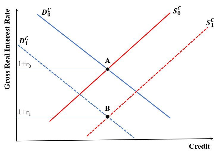
11Figure 3: Credit Market Equilibrium
Instead, we derive the total credit supply/saving
βλo λo νY
1
Stc = λ m am
t =λ m
(Y − D − T ) − , (7)
λm + βλo λ + βλo
m (1 + rt )
which depends on the length of middle age/working life and on the sub-period credit
supply/saving amt , by using (1), (2), (3), and (4). The effect of the PAYG pension
scheme on saving is twofold. First, the pension scheme decreases disposable income
and thus saving, for a given propensity to save, by levying T . Second, it provides
an income at old age, νY , that induces the household to save less by changing its
propensity to save. The negative effect of the PAYG scheme on saving reflects on the
gross equilibrium real interest rate,
(λm + βλo ) (1 + n) D + λo νY
1+r = , (8)
βλo (Y − D − T )
which would be lower without a pension scheme, that is for T = ν = 0. As depicted
in Figure 3, the credit demand Dtc relates negatively to 1 + r in (6), while the credit
supply/saving (7) relates positively to the real interest rate.8 Furthermore, a reduction
8
The relationship between saving and the real interest rate relies on the effect of a higher 1 + r on the
discounted value of future pension benefits. This relationship would not be necessarily positive with
12in the credit demand that shifts the corresponding curve downward, from D0C to D1C in
Figure 3, results in a lower equilibrium interest rate. The same happens for an increase
in the supply of saving, which shifts the credit supply curve downward, for example,
from S0C to S1C in the figure. On the contrary, an increase in the credit demand and
a decrease in saving would shift the corresponding curve upward, increasing the real
interest rate.
One last equation closes the model, the PAYG pension scheme budget constraint
Ntm λm T = Nto λo νY. (9)
The left-hand side (LHS) corresponds to the total contributions to the pension system,
while the right-hand side (RHS) is the total expenditure for pension benefits. On the
RHS, an increase in λo causes a higher expenditure for pensions because of a longer
Nm
retirement, while a lower fertility, 1+n = Nto , implies fewer middle-aged people relative
t
to retirees and so less contributions in aggregate.
2.2 Demographics, pension reforms and the natural interest
rate
We study the effects of demographics on the real interest rate, starting from an economy
where there is no pension system, i.e., T = ν = 0. Then, we introduce the PAYG
scheme and examine how the same demographic change affects r through alternative
pension reforms. As the purpose of this section is illustrative, we focus exclusively on a
permanent change in the duration of old age λo due to higher life expectancy, which is
the quantitatively most relevant demographic phenomenon taking place in the US. As
the credit demand, given by equation (6), is independent of λo , it is sufficient to study
the impact of λo on credit supply Stc to predict the implied change in the equilibrium
interest rate. Starting from the definition Stc = λm am
t in equation (7) and differentiating
o 9
with respect to λ , we get
∂Stc ∂λm m
m
∂am m
∂at t ∂λ
= a + + m λm . (10)
∂λo ∂λo t ∂λo ∂λ ∂λo
different preferences. Notwithstanding, we view the case considered as the most relevant empirically,
as Eggertsson et al. (2019).
m
9
Note that ∂λ
∂λo 6= 0 only when the government adjusts the retirement age in response to any change
in λo .
13In absence of the PAYG scheme, the effect of a higher life expectancy at old age is given
by
c N o−P AY G
βλm
∂St m
=λ (Y − D) > 0. (11)
∂λo (λm + βλo )2
A longer retirement increases savings via a higher propensity to save, and this, in turn,
translates in a lower equilibrium interest rate. For a given stock of wealth (1 + rt ) λm am
t ,
o
a higher λ reduces consumption in each sub-period of retirement in (3), inducing
middle-aged households to save more in each sub-period of working life. Demographic
factors, as well as affecting the incentives to save, carry important consequences for
λo N o
the pension system through the dependency ratio, DR = λm Ntm . As a result of longer
t
Nm
life expectancy, which causes higher λo , and/or lower fertility 1 + n = Nto , the DR
t
increases, undermining the financial sustainability of the public pension system. The
government can restore it by varying the policy parameters ν, T , λm and λo .
2.2.1 Reform of the replacement rate
If the government adjusts ν to offset the fiscal imbalance generated by demographic
phenomena, we get
Adjust−ν N o−P AY G
∂Stc ∂Stc βλm
1+n
= + m − 1 λm T > 0, (12)
∂λo ∂λo (λ + βλo )2 1+r
which is always positive.10 The replacement rate falls in response to an increase of
λo . Hence, lifetime income and old-age consumption decrease, forcing middle-aged
households to build up more saving each sub-period. The reform of the replacement
rate, induced by a longer life expectancy, amplifies the original effect of a higher λo on
saving, as shown by the last term on the RHS of the equation. This term also reveals
that in the presence of dynamic inefficiency, i.e., r < n, the credit supply response to a
10
Indeed, it can be alternatively written as
c Adjust−ν ( )
βλm
∂St m 1+n
∂λo
=λ 2 (Y − D − T ) + 1+r
T ,
(λm + βλo )
where (Y − D − T ) > 0 because the supply h of saving from middle-aged
i households has to be positive
m βλm 1+n
in presence of a PAYG. Only the term λ (λm +βλo )2 1+r T regards the reform of the replacement
h m
i c N o−P AY G
∂St
rate, while the term −λm (λmβλ+βλo ) 2 T , which does not enter ∂λo , arises because of the
presence of the pension scheme.
14change in ν is even stronger, because the return of the pension system is higher than the
return of the risk-free bond for each unit invested. To conclude, the endogenous decline
in ν puts further downward pressure on the equilibrium real interest rate through the
increase in saving.
2.2.2 Reform of the contribution
When, instead, the contribution to the pension scheme, T , changes in response to
adverse demographic trends, we obtain
Adjust−T N o−P AY G
∂Stc ∂Stc βλm λo βλo
νY 1+n
= − + + ,
∂λo ∂λo 1 + n (λm + βλo )2 λm + βλo 1+r
(13)
c N o−P AY G
∂St o
which is necessarily lower than ∂λo . A larger λ calls for an increase in
taxes, T when the replacement rate ν is unchanged. An increase in T incentivizes the
agent to optimally reduce savings, because the pension scheme pays the same benefit
νY and the decline in disposable income, Y − D − T , reduces the resources available for
consumption at middle-age. Overall savings Stc will increase or decrease depending on
whether the incentive to save due to a longer retirement period, in red, is stronger than
the disincentive implied by the pension system adjustment. This reform counteracts the
change in credit supply caused by demographic phenomena, mitigating the downward
pressure on the equilibrium interest rate r.
2.2.3 Reform of the retirement age
The reform of the retirement age (RA) alters the duration of working life and retirement,
λm and λo , so that their ratio returns to the level before the demographic change. This
fully neutralizes the impact of ageing on the pension scheme budget constraint:
λm νY
o
= . (14)
λ T (1 + n)
h i
∂am ∂am
t ∂λ
m
This reform implies that the term t
∂λo
+ ∂λm ∂λo
in equation (10) equals 0 because
λm
am
t only depends on the ratio λo
that remains constant. Therefore,
Adjust−RA
∂Stc λm m
= a > 0, (15)
∂λo λo t
15where we have implicitly assumed that the agent earns Y for each extra sub-period of
working life. The reform of the RA neutralizes the effect of ageing on the supply of
savings per sub-period amt due to an extended retirement period, (11), which disappears
in equation (15). However, the overall effect, direct and indirect through pensions, of
λo on Stc is positive because middle-aged agents save for more sub-periods, increasing
the total credit supply. Moreover, the variation in λm also increases credit demand (1)
putting upward pressure on r, therefore we cannot determine unambiguously the impact
of this reform on the equilibrium real interest rate. We now carry out a quantitative
analysis that, among the other things, can disentangle the net effect of the reform to
the RA on r.
163 Quantitative model
We develop a medium-scale life-cycle model to study the quantitative importance of
the pension channels, investigated theoretically in Section 2, for the past and future
evolution of the natural interest rate. The proposed theoretical framework draws on
the model in Eggertsson et al. (2019), with two substantial deviations. First, a public
PAYG pension system is explicitly modeled; second, a simple form of within-cohort
heterogeneity is introduced: only a fraction ψ < 1 of households for each cohort partic-
ipates to the scheme. These innovations allow accounting for the effect of pensions on
households’ saving decisions and better capture the specifics of the OASDI program in
the data.
In the remainder of this section, we briefly sketch out the behavior of households,
firms, and government. We put all the equations characterizing the model in the Ap-
pendix A, together with the definition of the competitive equilibrium and the outline
of the solution method.
3.1 Households
Households enter the economy and have kids at age 26, and they participate to the
labor market until their retirement at age RA. They die certainly at the maximum
possible age of J, which is 81 years, but they face a positive probability of dying even
before age J. The population growth depends on the fertility rate of every family, ft . A
representative household i aged j gets utility from consumption, ct (i, j), and from the
bequest left to each descendent, xt (i, j). The utility functions from consumption and
bequests, u(.) and v(.), are CRRA, and they are discounted at the rate β, multiplied by
the age-dependent survival probability sj . The elasticity of intertemporal substitution is
ρ, while the strength of the bequest motive is measured by the parameter µ. Households
leave bequests only at age J and receive inheritances, qt (j = 57), one period after the
death of their parents11 . Therefore, a household i entering the economy at time t
maximizes the lifetime utility
J
X
sj β j u ct+j−1 (i, j) + sJ β J µv xt+J−1 (i, J)
Ut (i) =
j=26
11
Formally, xt (i, j) = 0 ∀j 6= J and qt (j) = 0 ∀j 6= 57. As shown in the Appendix A.1, we
assume that inheritances qt do not depend on the index i, i.e., they are the same for participants and
non-participants to the pension system of the same age.
17subject to the budget constraints
h a (i, j) i
t
ct (i, j)+ξt at+1 (i, j+1) = (1−τtb −τtw 1i∈Ψt )wt hc(j)+Πt (j)+[rtk +ξt (1−δ)] +qt (j)
s(j)
h a (i, j) i
t
ct (i, j)+ξt at+1 (i, j +1)+ft−j+26 (26)xt (i, j) = pbt (j)1i∈Ψt +[rtk +ξt (1−δ)] +qt (j) .
s(j)
The first constraint holds for 26 ≤ j ≤ RA, when the household is young and active in
the labor market, while the second one holds for RA < j ≤ J, when the household is
old and retired. Households supply inelastically their labor endowment for the labor in-
come wt hc(j), where wt is the real wage and hc(j) is the age-dependent labor efficiency
level. A proportion τ b of the labor income is paid in form taxes to finance government
expenditure, while τ w is the contribution rate to the public pension system. The indica-
tor function 1i∈Ψt is a dummy that takes value 1 only when i ∈ Ψt , i.e., if the household
i participates to the public pension scheme, and it is 0 otherwise.12 The use of the
latter in the two budget constraints indicates that the pensions contributions/benefits
are paid/received only by participants. Young households also earn firms’ profits Πt (j),
which are distributed proportionally according to gross labor income.
Agents can save to smooth consumption over their lifetime by purchasing one-
period assets, at (i, j), in the form of physical capital or risk-free bonds. The exogenous
price of capital in consumption units is ξt , while the return on capital, which depreciates
at the rate δ, is rtk . Young households can also borrow, but they face a borrowing limit
of the form at (i, j)(1 + rt ) ≥ Dt (j) = dt wt hc(j), where 0 ≤ dt ≤ 1.13 Finally, all
households insure against the idiosyncratic risk of death before age J by participating
to annuity markets, as in Ríos-Rull (1996). Therefore, involuntary bequests are shared
among the surviving members of the same cohort, as expressed by the term ats(j) (i,j)
in the
two budget constraints. After retirement, individual income is the proceedings from
the investment decisions, and, for the public pension scheme participants, the pension
benefit pbt (j).
12
PJ
Ψt is the set of pension scheme participants at time t. The size of Ψt is ψt j=26 Nt (j), as a constant
fraction ψt of each cohort j participates to the public pension system .
13
For a no-arbitrage condition, the return from risk-free bonds equals that from capital investment:
1+rt = [rtk +(1−δ)ξt ]/ξt−1 . As regards the borrowing constraint, it is expressed on asset accumulation,
unlike that in equation (1) of the theoretical model. Moreover, Dt (j) grows at the rate of productivity
growth (due to wt ) and the household’s earning potential over the life-cycle (due to hc(j)).
183.2 Firms
The supply side of the economy is very rich, but it boils down to a few equations. For
all details and derivations, see Appendix A.2. The aggregate production function is
CES σ
σ−1 σ−1 σ−1
Yt = α(Ak Kt ) σ + (1 − α)(Al,t Lt ) σ ,
where Yt is aggregate output, σ is the elasticity of substitution between inputs, Al,t is a
labor-augmenting technological process growing at the exogenous rate gt , and Ak is the
capital productivity that is constant over time. Aggregate labor is the sum of the labor
productivity of each cohort weighted by its mass, Lt = Jj=26 Nt (j)hc(j).14 Moreover,
P
employers contribute to the pension system, along with their employees, and their tax
rate is τtf . However, not all workers participate to the pension system, so the total
contribution of firms is ψt τtf wt Lt . Aggregate capital Kt evolves over time according to
the law of motion Kt+1 = (1 − δ)Kt + ξItt , where It is aggregate investment and ξt is the
price of investment goods. Finally, the returns to capital and labor are, respectively
σ1
θt − 1 σ−1 Yt
rtK = αAk σ ,
θt Kt
σ1
1 θt − 1 σ−1 Yt
wt = f
(1 − α) Al,tσ ,
1 + ψt τt θt Lt
where θt > 1 is the elasticity of substitution across final good varieties.
3.3 Government
The government budget constraint is
Bt+1 = (1 + rt )Bt + Gt − Gpt − Tt ,
where Gt is the public expenditure, Gpt is the pension surplus, Bt denotes public debt,
and labor income taxes are Tt = τtb wt Lt . On the balanced growth path, we assume that
the government debt-to-output ratio is constant and the tax rate τ b varies to keep the
government budget balanced.15
14
After RA, hc(j) = 0.
15
This assumption implies that whenever Gpt < 0, the tax burden imposed by the pension deficit falls
on all working households, including those not covered by the public pension scheme. Similarly, if
193.4 Pension system
The pension system plays a central role in our quantitative model, and we tailor it to
replicate the salient features of the US public pension system, the OASDI program.
While a fraction of households, ψ < 1, participates to the public pension system,
contributing the tax rate τ w when working and receiving the pension pbt (j) once retired,
the remaining fraction of households does not, τ w = pbt (j) = 0. The budget constraint
of the pension system is
RA
X J
X
Gpt = ψτtp wt Nt (j)hc(j) − Nt (j)pbt (j), (16)
j=26 j=RA+1
where τtp = τtw + τtf is the total contribution rate from workers and employers. The
first term on the RHS is the total contribution from working households, while the
second term is the total expenditure for pensions benefits to retirees. Equation (16) is
the equivalent of (9) in the theoretical model. However, now the pension budget is not
necessarily balanced. The variable Gpt denotes the pension system surplus or deficit,
depending on whether the total contributions exceed the total benefits or vice versa.
This new assumption allows for more precise calibration of the model to the OASDI
program, which has run a surplus over the last decades but it is expected to undergo
deterioration of its financial conditions due to population ageing.
The financial balance of the pension system crucially depends on how the policy
parameters, τtp , RA, and the replacement rate νt , adjust to the demographic pattern.
The individual pension benefit of a retiree aged j is:
RA
wt−j+60 X
pbt (j) = νt φ(RA, F RA) hc(z). (17)
35 z=RA−35+1
Our calculation of the pension benefit, which is a fraction νt of the average gross labor
income, follows the US Social Security regulation closely. A detailed account of the
computation procedure can be found in Appendix A.3. In short, the US Social Secu-
rity Administration computes the pension benefits according to the Primary Insurance
Amount (PIA), which considers only the average labor earnings of the top 35 years of
contribution, defined as Average Indexed Monthly Earnings (AIME). Monthly earnings
are indexed relative to the average wages of the indexing year, the year in which the
Gpt > 0, the pension surplus is shared across all working households.
20contributor turns 60. We calculate the AIME by averaging the gross labor earnings
of the last 35 years of work because, given the calibration, they correspond to the top
35 years of earnings. On the other hand, we index individual wages relative to the
economy-average wage in the year in which the agent turned 60, i.e., wt−j+60 . As the
US regulation applies a penalty to benefits in case of early retirement, the function
0 < φ(RA(i), F RA) ≤ 1 gives the penalty, in terms of replaced contributions, if the
individually chosen retirement age RA(i) is lower than the full retirement age F RA.
21Table 1: Calibration
Parameters Symbol 1970 value 2015 value
Parameters estimated directly from the data Source
Mortality profile sj US mortality tables, CDC
Income profile hcj Gourinchas and Parker (2002)
Total fertility rate n 2.8 1.88 UN fertility data
Productivity growth g 2.02% 0.65% Fernald (2012)
Government spending (percent of GDP) G 21.3% 21.3% CEA
Public debt (percent of GDP) b 42% 118% Flow of Funds
Retirement age RA 63 65 US Census Bureau
Replacement rate ν 32.3% 40.8% US Social Security
OASDI program coverage 90% 96% US Social Security
Pension contribution rate τp 8.4% 12.4% US Social Security
Parameters taken from the literature Source
Elasticity of intertemporal substitution ρ 0.75 0.75 Gourinchas and Parker (2002)
Capital/labor elasticity of substitution σ 0.6 0.6 Antras (2004)
Depreciation rate δ 12% 12% Jorgenson (1996)
Price of investment goods ξ 1.3 1 Fernald (2012)
Parameters calibrated matching some data moments
Rate of time preference β 0.96 1.005
Borrowing limit (percent of annual gross labor income) d 9.52% 50.22%
Bequests parameter µ 55.06 9.12
Retailer elasticity of substitution θ 8.6 4.89
Capital share parameter α 0.19 0.24
Data moments Source
Natural rate of interest 2.62% -1.47% FED
Investment-to output ratio 16.8% 15.9% NIPA
Consumer-debt-to-output ratio 4.2% 6.3% Flow of Funds
Labor share 72.4% 66% Elsby et al. (2013)
Bequests-to-output ratio 3% 3% Hendricks (2002)
224 The natural interest rate in the past
We employ our quantitative model to study the importance of several determinants
of the declining trend, between 1970 and 2015, in the US natural interest rate. We
emphasize the role of the pension system and its interaction with demographic and
productivity changes, because we aim to verify whether the pension system matters
for the past pattern of the natural interest rate. Our positive analysis consists of
comparative statics between balanced growth path-stationary equilibria, and we assume
a zero output gap in 2015 so that the natural and real interest rates coincide, at -1.47%,
and the two terms can be used interchangeably.16
As we have drawn on the life-cycle model of Eggertsson et al. (2019) for the
construction of our quantitative framework and augmented it with a realistic pension
system, we treat their model as a benchmark to highlight the specific effect of the pen-
sion system on the natural interest rate. Moreover, as our calibration procedure follows
closely that in Eggertsson et al. (2019), we focus only on the calibration of the parame-
ters governing the pension system, referring the reader to that paper for further details.
Table 1 summarizes our calibration. The first set of parameters, including pension pa-
rameters, are directly estimated from data. We take the second set of parameters from
the related literature. We internally calibrate the parameters in the third set to match
some key moments in data by minimizing a quadratic loss function.
The US Social Security regulation established that the FRA was around 66 years
in 2015, but early retirement was possible at 62 years. To take into account the effect
of early retirement, we calibrate the effective RA at 65, which is slightly lower than
66 and is consistent with Eggertsson et al. (2019). Regarding 1970, we opt for a more
conservative calibration of the RA, 63 years, against the average RA of roughly 65 years
for men (US Census Bureau).17 However, we perform a robustness check in Appendix
B.1, where we assume a higher RA in 1970, 64 years, and so a lower variation in the
RA over the period 1970-2015. Given our calibration of the RA in 1970 and 2015, our
formula for calculating the pension benefits, (17), implies a reduction of 13.3% of the
16
Although there are several and different estimates of the US’s output gap after the Great Recession;
we base our assumption of zero output gap on Stock and Watson (2012).
17
In 1970, there was a large fraction of women excluded from the official labor force. Although data
on the average retirement for men are available, average statistics can be misleading because of a
left-skewed distribution. Moreover, the so-called survivorship bias and the decision to retire early
of sick people significantly affect the data. These are the considerations motivating our conservative
calibration for the RA in 1970.
23replacement rate for early retirement in 1970 and 6.66% in 2015.
The contribution rate for the OASDI in 1970 was 4.2% of the gross labor income
for both employer and employee, while it was 6.2% in 2015. Hence, τ p = τ w + τ f
is 8.4% in 1970 and 12.4% in 2015. We calibrate the replacement rate using the US
Social Security Administration data on the medium earner’s pension benefit, whose net
replacement rate was around 32.3% in 1970 and approximately 40.8% in 2015.18 The
positive variation in the replacement rate is a sign that the program experienced an
increase in its generosity over the period considered. Hence, we expect it to have miti-
gated the secular fall in the natural interest rate. Such reform seems to respond more
to pension adequacy considerations rather than to the problem of pension funding. In
the last fifty years, the US population has experienced adverse demographic dynamics,
which were less pronounced than those of other advanced economies. Consequently,
the financial sustainability of the public pension scheme was overall less of a pressing
concern. Finally, the OASDI program underwent a substantial expansion in terms of
coverage, as documented in the historical accounts of the US Social Security Admin-
istration. While in 1970 Social Security involved around 90% of civilian workers, this
proportion increased to 96% in 2015.
18
Data available at https://www.ssa.gov/oact/NOTES/ran9/index.html.
24Table 2: Decomposition of the decline in the natural interest rate
Forcing variable Our results EMR (2019)
Total real interest rate variation -4.09% -4.02%
Single effect
Mortality rate -0.64% -1.82%
Total fertility rate -0.38% -1.84%
Productivity growth -1.44% -1.90%
Government debt (percent of GDP) +0.99% +2.11%
Relative price of investment goods -0.27% -0.44%
Replacement rate +0.50% -
Retirement age +0.44% -
Contribution rate -0.05% -
Coverage +0.16% -
Combined effect
All pension adjustments +1.10% -
Mortality + Fertility -0.99% -
Mortality + Fertility + Replacement rate -0.71% -
Mortality + Fertility + Retirement age -0.59% -
Mortality + Fertility + Contribution rate -1.02% -
Mortality + Fertility + Coverage -0.90% -
Mortality + Fertility + all pension adjustments -0.21% -
Demographics + pension adjustments + productivity slowdown -1.90% -
Demographics + productivity slowdown -2.69% -
254.1 Results
We decompose the decline in the US natural interest rate, denoted by r∗ hereafter,
among all its potential drivers through the following procedure. We treat 1970 and 2015
as two balanced growth path-stationary equilibria, and we calibrate our quantitative
model accordingly. We first take the 2015 stationary equilibrium. Then, we shock, one
at a time, the parameters associated with the drivers of r∗ assigning them the value
they take in the 1970 equilibrium, keeping all the other parameters constant. Finally,
we interpret the implied variation in the real interest rate as the single driver’s effect
on the evolution of r∗ over 1970-2015. If the implied variation is positive, the driver’s
effect is negative and vice versa for a negative variation. The top part of Table 2 shows
the results of our decomposition for the single drivers, that is the “single effect”. Our
quantitative model accounts for the full decline of -4.09 percentage points, from 2.62%
in 1970 to -1.47% in 2015, in r∗ . In particular, it delivers three key results.
First, the public pension scheme matters, in a static sense (i.e. absent any pension
adjustment over time) to quantify the impact of all the potential drivers of the decline in
r∗ , as accounting for it determines a different calibration of the model parameters. The
decrease in the mortality and fertility rates, the productivity slowdown, and the surge
in government debt still qualify as the main drivers of the past pattern of the natural
interest rate. But their quantitative impact falls greatly in absolute value, compared
to Eggertsson et al. (2019), once the model accounts for the pension system and its
evolution between 1970 and 2015. Taking as an example the demographic phenomena,
the fall in the mortality rate has negatively impacted the natural interest rate just by
64 basis points, against the 182 basis points originally obtained in Eggertsson et al.
(2019). The drop in the total fertility rate pushes r∗ down by 38 basis points, while
the original effect was -184 basis points. The first quantitative finding derives from the
pension system’s ability to absorb savings and raise the natural interest rate, as well as
its implications for the calibration of the model.
In this sense, we interpret the discrepancies in results relative to Eggertsson et
al. (2019) as a consequence of the role of the public PAYG system for the saving
behavior and its differences, as an asset, with respect to the bonds and capital in the
model. Contributing to the pension scheme reduces disposable income and crowds out
private savings and bequests. Moreover, the PAYG entitlement offers a different type of
insurance relative to the other assets in the model. Its overall return increases with the
individual household’s life span, favoring/hurting those that, ex-post, die later/earlier
26than the economy life-expectancy at birth. Instead, the assumption of perfect annuity
markets for private savings grants intra-cohort insurance against the age-specific risk
of death.
Second, the pension system matters, in a dynamic sense, because the effect of
the observed pension reforms on the natural interest rate is positive and quantitatively
significant. As well as to measure the single driver’s impact on the pattern of r∗ , we
also consider several drivers simultaneously, that is the “combined effect”, such as all the
pension reforms implemented. The bottom part of Table 2 shows that the changes to
replacement and contribution rates, RA, and coverage have counteracted the downward
pressure of the other forces on r∗ , raising the natural interest rate by approximately
1% overall.
When we consider every single reform in the top part of Table 2, the change
in the replacement rate plays the most significant role. This result is not striking
because the replacement rate has increased from 32.3% to 40.8%, over the period under
investigation, discouraging private savings and increasing r∗ by 0.5 percentage points.
The quantitative impact of a higher RA is similar, +0.44 percentage points, and this
is because each household spends a slightly larger fraction of her lifetime working and
needs fewer savings to support the same amount of consumption at old age.19 In
Appendix B.1, an alternative calibration of the model featuring a lower increase in the
RA confirms this result qualitatively (the sign). However, the alternative calibration
points to a smaller quantitative impact of a higher RA on r∗ , +12 basis points, while the
overall effect of all pension reforms is still significantly high, +0.77 percentage points.
Finally, the effect of a higher coverage on the natural interest rate is small, but not
negligible. At the same time, the impact of the pension contributions is very close to 0
because the change in τ p is marginal.
Third, the pension system matters for the evolution of the natural interest rate
because of its dynamic interaction with demographic and technological trends. In the
bottom part of Table 2, we measure first the simultaneous effect of pension reforms
and changes in the fertility and mortality rates; then, we also consider the slowdown in
productivity that occurred between 1970 and 2015. Demographics alone explains a fall
in r∗ of about one percentage point, which becomes -2.7 percentage points if we take
into account also the productivity change. When we consider all the pension reforms in
19
PJ
Ceteris paribus, a higher RA increases the aggregate labor supply, Lt = j=26 Nt (j)hc(j) for positive
levels of labor productivity around RA. Given the CES technology, a larger Lt increases rtK for the
same amount of capital.
27conjunction with both demographic shocks, the real interest rate drops just by 21 basis
points, while the fall is -190 basis points if we add the productivity decline. Again, the
single pension reforms that drive these results are the reform to the replacement rate
and the RA.
To summarize, our quantitative results highlight a positive effect of the US pension
system on the past evolution of the natural interest rate. The capacity of the public
pension scheme to exert upward pressure on r∗ is particularly significant because it
counteracts the downward pressure from adverse demographic and technological trends.
Notwithstanding, the positive effect relies mainly on the increase in the replacement
rate possible because of more favorable demographic trends than in other advanced
economies. In the future, more adverse demographic patterns resulting in a higher DR
could make a further increase in the replacement rate highly costly, and demographics
itself could become so pronounced to push r∗ further down. The future evolution of the
natural interest rate is at the center of the next section.
5 The natural interest rate in the future
We use the same model of the previous section for a prospective analysis, in which we
simulate the future demographic dynamics under two opposite productivity scenarios
to evaluate the impact of different pension reforms on r∗ and welfare. Specifically, we
structure our normative exercise as follows.
We simulate the US economy’s transition dynamics in response to the future de-
mographic trends, estimated by the UN between 2015 and 2060, taking as a starting
point the 2015 stationary equilibrium. In 2016, the economy is shocked unexpectedly by
changes in mortality, fertility, and production growth. From 2016 onward, agents have
perfect foresight of the evolution of productivity, pension adjustments and demographic
variables, which return constant after 2060, when the economy starts to converge to
a new stationary equilibrium.20 Moreover, we inform the model with the available
estimates of demographic trends between 2015 and 2060, including year-by-year age-
dependent survival probabilities and fertility rates. This setting allows us to study
the natural interest rate and the welfare of all the generations involved in the transi-
20
All agents older than 26 years are surprised by the shocks in 2016, and they revise their optimal
decisions of consumption and saving over the life-cycle. Instead, cohorts entering the economy after
that have full information on the evolution of prices and pension benefits, and they make their decisions
accordingly.
28You can also read