Railway Commuting Costs and Housing Prices in Norway: an Empirical Analysis
←
→
Page content transcription
If your browser does not render page correctly, please read the page content below
Railway Commuting Costs and Housing Prices
             in Norway: an Empirical Analysis

                 Haakon Gjersum and Per Stefan Præsterud

                                         2017

                                    MASTER THESIS
                                Department of Economics
                  Norwegian University of Science and Technology

Supervisor 1: Professor Kåre Johansen
Supervisor 2: Patrick Ranheim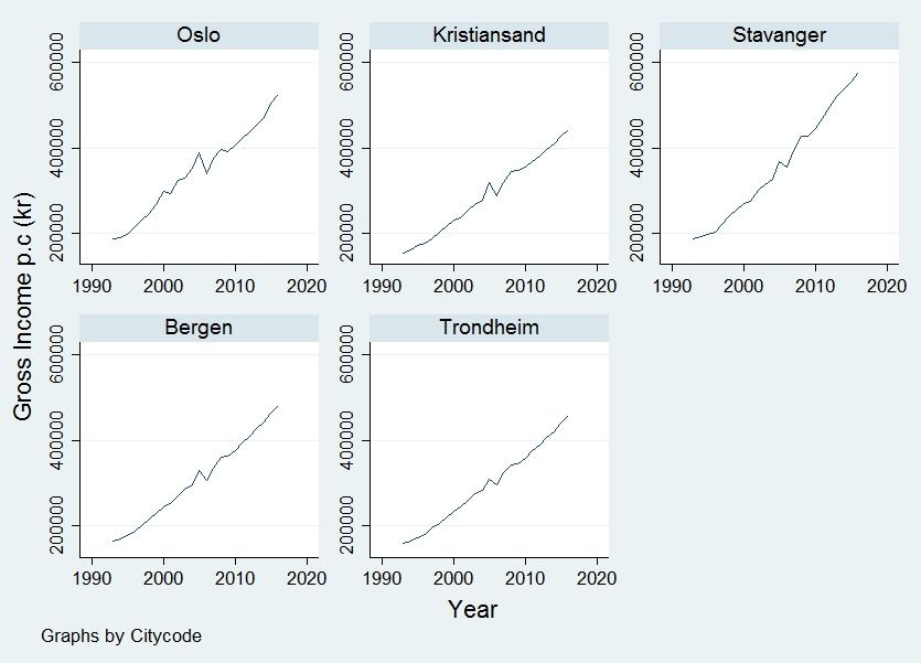
ii

Preface
This thesis is a part of our masters degree in economics at the Norwegian University of Science and
Technology. The thesis is written in collaboration with The Norwegian Railway Directorate.

We would like to thank our supervisors, professor Kåre Johansen at the Department of Economics
at NTNU and Patrick Ranheim, at the Norwegian Railway Directorate, for helpful inputs and guid-
ance. We would also like to thank Wendy G. Bemrose for proofreading and Tora Uhrn for illustra-
tions.

The master thesis is a joint work performed by Haakon Gjersum and Per Stefan Præsterud. Any
mistake is our own and we take full responsibility for its content.

                                      Trondheim, 2017-06-01

                             (Haakon Gjersum, Per Stefan Præsterud)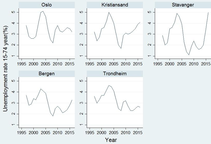
iv

Abstract
In this thesis we present a new variable measuring the generalised time costs of commuting to and
from central municipalities in Norway, from 1997 to 2016. We use this variable to estimate the
effect of changes in railway transportation quality on housing prices in the central municipalities.
The empirical analysis is performed by using a fixed effects regression model based on data for five
of Norway’s biggest municipalities; Oslo, Kristiansand, Stavanger, Bergen and Trondheim. We ap-
ply both static and dynamic models. We find that the generalised time costs of railway commuting
has decreased in all municipalities between 1997 and 2016. Average commuting costs is highest in
Bergen and lowest in Oslo. We find evidence of an inverse relationship between railway commut-
ing quality to and from the central municipalities and housing prices within the municipalities. The
short-run elasticity of housing prices with respect to changes in generalised time costs of commut-
ing is about 0.2 per cent, while the long-run elasticity is about 0.4 per cent.

Keywords: housing prices; housing price dynamics; fixed effects; generalised time costs; trans-
port economy; railway commuting.
Contents

    Preface . . . . . . . . . . . . . . . . . . . . . . . . . . . . . . . . . . . . . . . . . . . .   ii
    Abstract . . . . . . . . . . . . . . . . . . . . . . . . . . . . . . . . . . . . . . . . . . .    iv

1   Introduction                                                                                       1

2   Literature Review of Housing Prices                                                                5
    2.1    Modelling Housing Prices . . . . . . . . . . . . . . . . . . . . . . . . . . . . . .        5
    2.2    Effects of Transport Quality on Housing Prices . . . . . . . . . . . . . . . . . . .        6

3   Theory                                                                                            9
    3.1    Consumer Theory with Durable Goods . . . . . . . . . . . . . . . . . . . . . . . .          9
    3.2    Aggregation and Total Demand . . . . . . . . . . . . . . . . . . . . . . . . . . . .       12
    3.3    Housing Market Equillibrium . . . . . . . . . . . . . . . . . . . . . . . . . . . . .      14
    3.4    Generalised Costs . . . . . . . . . . . . . . . . . . . . . . . . . . . . . . . . . . .    18

4   Data                                                                                              19
    4.1    Housing Prices . . . . . . . . . . . . . . . . . . . . . . . . . . . . . . . . . . . .     19
    4.2    Gross Income . . . . . . . . . . . . . . . . . . . . . . . . . . . . . . . . . . . . .     21
    4.3    Unemployment Rate . . . . . . . . . . . . . . . . . . . . . . . . . . . . . . . . .        23
    4.4    Generalised Time Cost of Commuting . . . . . . . . . . . . . . . . . . . . . . . .         25
           4.4.1   Converting NSB Time Tables . . . . . . . . . . . . . . . . . . . . . . . .         26
           4.4.2   Trenklin III . . . . . . . . . . . . . . . . . . . . . . . . . . . . . . . . . .   27
           4.4.3   Calculating The Average Generalised Time Cost for Each City . . . . . . .          29
    4.5    Descriptive Statistics . . . . . . . . . . . . . . . . . . . . . . . . . . . . . . . . .   33

                                                   vi
CONTENTS vii
5 Empirical Specification 35
5.1 Baseline Model . . . . . . . . . . . . . . . . . . . . . . . . . . . . . . . . . . . . 35
5.2 Time Fixed Effects . . . . . . . . . . . . . . . . . . . . . . . . . . . . . . . . . . 37
5.3 Housing Market Dynamics . . . . . . . . . . . . . . . . . . . . . . . . . . . . . . 38
5.4 Serial Correlation and Driscoll and Kraay Standard Errors . . . . . . . . . . . . . 39
5.5 Measurement Errors . . . . . . . . . . . . . . . . . . . . . . . . . . . . . . . . . . 40
6 Results 42
6.1 Static Housing Price Model . . . . . . . . . . . . . . . . . . . . . . . . . . . . . . 42
6.2 Housing Price Dynamics . . . . . . . . . . . . . . . . . . . . . . . . . . . . . . . 44
6.3 Effects of Generalised Time Costs on 2016 Housing Prices . . . . . . . . . . . . . 46
6.4 Alternative Functional Forms and Non-linearity . . . . . . . . . . . . . . . . . . . 49
6.5 Summary of Results . . . . . . . . . . . . . . . . . . . . . . . . . . . . . . . . . . 54
7 Conclusion 56
Bibliography 60
A Additional Information i
A.1 Estimation Gross Income 2016 . . . . . . . . . . . . . . . . . . . . . . . . . . . . i
A.2 The Process of Making the Generalised Time Costs Variable . . . . . . . . . . . . i
A.2.1 Trenklin Transport Matrices . . . . . . . . . . . . . . . . . . . . . . . . . i
A.2.2 Intepretation of the Generalised Time Cost Matrix . . . . . . . . . . . . . v
A.3 Assumptions with Fixed Effects and Random Effects Models . . . . . . . . . . . . vi
A.4 Unit Root Test . . . . . . . . . . . . . . . . . . . . . . . . . . . . . . . . . . . . . vii
A.4.1 Log Housing Prices . . . . . . . . . . . . . . . . . . . . . . . . . . . . . . viii
A.4.2 Log Unemployment . . . . . . . . . . . . . . . . . . . . . . . . . . . . . ix
A.4.3 Log Gross Income . . . . . . . . . . . . . . . . . . . . . . . . . . . . . . ix
A.4.4 Log PGC2 . . . . . . . . . . . . . . . . . . . . . . . . . . . . . . . . . . x
A.5 Durbin’s Test for Serial Correlation With Strictly Exogenous Regressors . . . . . . x
A.6 Durbin’s Test for Serial Correlation Without Strictly Exogenous Regressors . . . . xi
A.7 Testing Hypotheses About a Single Population Parameter: The t-test . . . . . . . . xiiiList of Figures
3.1 Housing Market Equillibrium . . . . . . . . . . . . . . . . . . . . . . . . . . . . . 15
3.2 Generalised Time Costs and Population . . . . . . . . . . . . . . . . . . . . . . . 16
3.3 Housing Demand Shift . . . . . . . . . . . . . . . . . . . . . . . . . . . . . . . . 17
4.1 Development in Housing Prices 1992-2016 . . . . . . . . . . . . . . . . . . . . . 20
4.2 Gross Income . . . . . . . . . . . . . . . . . . . . . . . . . . . . . . . . . . . . . 22
4.3 Development in Unemployment Rate 1999-2016 . . . . . . . . . . . . . . . . . . 24
4.4 PGC Flow Chart . . . . . . . . . . . . . . . . . . . . . . . . . . . . . . . . . . . . 26
4.5 Day-distribution of Travels Used in Thesis . . . . . . . . . . . . . . . . . . . . . . 29
4.6 Central Municipalities and Commuting Radiuses . . . . . . . . . . . . . . . . . . 30
4.7 PGC . . . . . . . . . . . . . . . . . . . . . . . . . . . . . . . . . . . . . . . . . . 31
6.1 Observed Change in Housing Prices and Share Explained by PGC2 . . . . . . . . 48
6.2 Estimated Relationship Between PGC2 and lHp in Model(3) . . . . . . . . . . . . 51
6.3 Estimated Relationship Between PGC2 and lHp in Model(4) . . . . . . . . . . . . 52
A.1 Time Cost of Waiting . . . . . . . . . . . . . . . . . . . . . . . . . . . . . . . . . iii
ixList of Tables
4.1 Housing Prices . . . . . . . . . . . . . . . . . . . . . . . . . . . . . . . . . . . . 21
4.2 Average Gross Income . . . . . . . . . . . . . . . . . . . . . . . . . . . . . . . . 22
4.3 Unemployment Rate . . . . . . . . . . . . . . . . . . . . . . . . . . . . . . . . . 25
4.4 Timetable Entries . . . . . . . . . . . . . . . . . . . . . . . . . . . . . . . . . . . 27
4.5 Descriptive Statistics PGC2(minutes) . . . . . . . . . . . . . . . . . . . . . . . . 32
4.6 Descriptive Statistics PGC1(minutes) . . . . . . . . . . . . . . . . . . . . . . . . 32
4.7 Descriptive Statistics . . . . . . . . . . . . . . . . . . . . . . . . . . . . . . . . . 33
6.1 Fixed Effects Estimates With Driscoll and Kraay Robust Standard Errors . . . . . . 43
6.2 Change in 2016 Housing Prices With a 1 Percent Increase in PGC2, 95%-Confidence
Interval . . . . . . . . . . . . . . . . . . . . . . . . . . . . . . . . . . . . . . . . 44
6.3 Fixed Effects Estimates with Driscoll and Kraay Robust Standard Errors Dynamic
Model . . . . . . . . . . . . . . . . . . . . . . . . . . . . . . . . . . . . . . . . . 45
6.4 Summary of the Effects on Housing Prices with Lower Transport Quality . . . . . 46
6.5 Housing Price and PGC2 Variation . . . . . . . . . . . . . . . . . . . . . . . . . . 47
6.6 Effect of one Standard Deviation Railway Quality Improvement . . . . . . . . . . 47
6.7 Dynamic Model Estimation with Non-linearity . . . . . . . . . . . . . . . . . . . 50
6.8 Comprehensive Model . . . . . . . . . . . . . . . . . . . . . . . . . . . . . . . . 53
6.9 Test of Nonnested Models . . . . . . . . . . . . . . . . . . . . . . . . . . . . . . 54
A.1 Average Waiting Time on Station Oslo S-Fredrikstad 2016 . . . . . . . . . . . . . iii
A.2 Average On Board Time Oslo S-Fredrikstad 2016 . . . . . . . . . . . . . . . . . . iv
A.3 Average Transfers Oslo S-Fredrikstad 2016 . . . . . . . . . . . . . . . . . . . . . iv
xiLIST OF TABLES 1 A.4 Average Waiting Time on Transfers Oslo S-Fredrikstad 2016 . . . . . . . . . . . . v A.5 Generalized Costs Oslo S-Fredrikstad . . . . . . . . . . . . . . . . . . . . . . . . v A.6 LLC Unit Root Test for lHp . . . . . . . . . . . . . . . . . . . . . . . . . . . . . . viii A.7 LLC Unit Root Test for lunem . . . . . . . . . . . . . . . . . . . . . . . . . . . . ix A.8 LLC Unit Root Test for lY . . . . . . . . . . . . . . . . . . . . . . . . . . . . . . ix A.9 LLC Unit Root Test for lPGC2 . . . . . . . . . . . . . . . . . . . . . . . . . . . . x A.10 AR(1) Serial Correlation Test . . . . . . . . . . . . . . . . . . . . . . . . . . . . . xi
Chapter 1

Introduction

In this thesis we pose the question; Does improvements in railway quality for commuters diminish
the housing price inflation in central municipalities in Norway? We aim to estimate a relationship
between housing prices and variations in the time costs of travelling, also known as generalised
time costs. The mechanism behind our hypothesis is the following; better railway quality for work
commuters will increase the attractiveness of living in more peripheral areas relative to the central
municipality, and thereby reducing its population. All else equal, a lower population in central city
areas implies lower aggregate demand for housing and less pressure on housing prices.
   The Norwegian housing market is an interesting subject with a broad specter of analyses to un-
derstand its developments. From Anundsen and Jansen (2011) estimating the interaction between
housing prices and household borrowing, to Fiva and Kirkebøen (2011) which looks at housing
market reactions to published school quality reports. Eide (2015) investigates the connection be-
tween taxation and housing prices. All in all, there is a lot of focus on this area.
   As the data will show, all major cities in Norway have experienced substantial rising housing
prices over the past two decades. The development of housing prices in the major cities is also
evident in the rest of Scandinavia. According to Norges Bank (2016), all Scandinavian countries
have experienced a larger increase in housing prices in their major cities compared to the respec-
tive country overall. After the global financial crisis in 2008 and the following drop in the oil
price in 2014, Norway has also experienced a rise in unemployment and lower investments. These
two effects, coupled with a rising housing market and credit growth, has presented policy makers
with a dilemma between financial stability and counter-cyclical monetary policy. This makes the

                                                   1
CHAPTER 1. INTRODUCTION 2
developments and drivers in the housing market an important issue for analysis.
In the early 2000s, Norway lagged behind other major cities on the European continent in terms
of centralisation and migration trends. Østby (2001) discusses how Norway was still characterised
by a great deal of urbanisation, and points out that international studies found Norway to differ
from other European cities, where centralisation declined in the 1990’s. Brunborg (2009) states
that such migration trends in Norway continued towards 2009 and that the population share living
in the most central municipalities, has increased from 61 to 67 percent from 1980 to 2009. It is
reasonable to believe that these migration trends have contributed to the rising housing prices seen
in the major cities in Norway. Around central cities and municipalities, people balance the decision
between migration and commuting. Improving the railway quality for commuters to and from the
central municipalities can enhance commuting as an alternative to migration, and reduce demand
and housing prices in the central municipalities. Holvad and Preston (2005) finds that reduced
commuting costs, caused by improved transportation infrastructure, can influence commuting and
migration decisions. Commuters can travel longer stretches for the same amount of generalised
time costs, leading to higher migration to areas with lower housing prices. They also argue that
inflating housing prices in a region, which is a net importer of labor, could give commuting rather
than migration to the district.
Our contribution to this subject is the construction of a generalised time cost variable for railway
commuting. The variable illustrates the development in railway quality in Norway for the past
20 years. We will use this variable to explain the link between the costs of commuting to and
from central municipalities and housing prices in these municipalities. The generalised time cost
variable is generated based on railway quality components between the central stations in central
municipalities in Norway, and stations outside the cities’ municipality border. To isolate the railway
quality improvements relevant for commuting to and from the municipality, we exclude the stations
within the municipality border.
In a world with a continually growing population and limited land resources, urban structure
and land use will become increasingly important in the future. In the National Transport Plan
(NTP) for 2018-20291 , the Norwegian government assumes a population growth of about 1 percent
1
See Norwegian Railway Directorate, Norwegian Coastal Administration and Norwegian Public Roads Adminis-
tration (2017)CHAPTER 1. INTRODUCTION 3
per year from 2016 to 2022. This implies a population of over 5.5 million people in 2022. The
transport plan outlines how the Government intends to prioritise the transport sector over a twelve
year period. One of the objectives in the NTP is the ”Zero growth objective”, this implies that,
excluding cycling and walking, the growth in passenger transport in the cities is to be absorbed by
public transportation. The Norwegian Ministry of Transport and Communications states that2 :
”Together with other public transportation options, the train will contribute to improved ac-
cessibility in the metropolitan areas. The development of modern rail infrastructure between cities
and towns provides reduced travel times, frequent and regular departures and better punctuality.
This means that people can choose to live and work where they want and larger areas are linked to
a common housing and labor market”.
The statement underlines the relevance of future railway commuting. This leads the way for an
interesting analysis of the link between railway transportation quality for commuters and aggregate
housing demand and housing prices in the central municipalities. In this thesis we investigate the
link empirically, using five central municipalities in Norway; Oslo, Kristiansand, Stavanger, Bergen
and Trondheim.
The structure of the thesis is: Chapter 2 will provide relevant earlier literature and chapter 3
presents economic theory. In chapter 4 we describe the data and the process of calculating the gen-
eralised time costs variable. Chapter 5 explains the empirical specification and chapter 6 presents
the empirical results. Chapter 7 concludes.
2
See Transport Communications Ministry (2015)Chapter 2
Literature Review of Housing Prices
The development in housing prices has been a popular subject for theoretical and empirical analysis
over the past few years. In our research for this thesis we have encountered numerous national and
international papers trying to explain the movements in housing prices. In this section we will
review some of the literature regarding housing prices with respect to variables and methods of
interest.
2.1 Modelling Housing Prices
In this thesis we use unemployment and income as control variables when estimating the effect
of commuting costs on housing prices. Income and unemployment affect the attractability of the
municipalities and affect aggregate housing demand. Arestis and Gonzales (2013) from the Levy
Economics Institute models the housing price developments in 18 OECD countries from 1970
to 2011 using a vector error correction model (VECM). A VECM is a time-series model used
for data with a cointegrating relationship between the underlying variables. The authors point to
disposable income as the cornerstone of their model. In addition to disposable income, they model
housing prices as a function of residential investment, banking credit, mortgage rate, taxation,
unemployment and population. Their analysis focuses on both a long-run relationship as well as
short-run dynamics, keeping housing supply fixed in the short run. Their empirical findings for
the short run is that previous levels of real housing prices plays a significant role in explaining
the development of housing prices in Norway. This is, as underlined by Asteris and Gonzales,
5CHAPTER 2. LITERATURE REVIEW OF HOUSING PRICES 6 an effect of the role of expectations and speculation in the housing market. Additional findings for Norway include that unemployment is not relevant in explaining the short-run dynamics, but population is. Our analysis will build upon some of the same variables as Asteris and Gonzales. We will use income and unemployment as control variables to explain migration decisions and changes in aggregate housing demand in each municipality. Macro economic variables that vary over time, such as interest rates, also affect housing demand. Because all our entities are cities within the same country, these variables do not vary between entities and can be controlled for with econometric techniques. 2.2 Effects of Transport Quality on Housing Prices Kulish et al. (2012) investigates the development of urban structure and housing prices in Aus- tralia. They apply a basic model of Alonso(1964), Muth(1969) and Mills(1967), which assumes a city with fixed population and a given income level. The population lives around a central business district(CBD) and travel into the city center for work. Since commuting is costly and increases with the distance to the CBD, households would choose to live closer to the city center. The model assumes, as we do in this thesis, that households are identical in preferences. Their empirical anal- ysis points to the potential significance of transport infrastructure. This includes public transport infrastructure as well as infrastructure for cars. The authors calibrate transport costs a monetary cost as well as a time cost. The time cost is valued to 60 percent of the wage rate. The remain- der is assumed to be spent on housing and other goods. This means that higher income leads to higher time costs. They find that in cities with better transport infrastructure, it is more feasible to live further away from the city where housing prices are lower, because of lower commuting costs. This supports the theory that improvement in transportation infrastructure to central business areas can reduce aggregate housing demand in the city. In relevance to our thesis, this would imply that better railway infrastructure, to for example Trondheim from Stjørdal, could reduce housing price pressure in Trondheim city. Lower commuting costs on the railway line from Stjørdal to Trondheim could make it more feasible to live in Stjørdal, 33 kilometers north-east of Trondheim. Grue et al. (1997) uses the log of housing prices in a hedonic pricing model for houses in three regions around Oslo city centre. These regions are Oslo West, Grorudalen-Østensjø and
CHAPTER 2. LITERATURE REVIEW OF HOUSING PRICES                                                       7

North-South. A hedonic model treats housing as a heterogeneous good where its value depends
on different attributes of the houses(i.e. floor-space, age, number of rooms etc.). In our analysis
we treat housing as a homogenous good and use variables affecting aggregate demand to model
changes in housing prices. In Grue et al. (1997), the main focus of the analysis is on the exposure
to road traffic as measured by outdoor noise levels and location in terms of distance from city
center. The contributions of a number of additional variables are also estimated. One of these is
the measure of the public transportation quality in form of generalised costs per kilometer distance
to the city center. Their empirical analysis is based on two seperate datasets. One from 1995 with
condominium apartments and a second from 1988-1995 with flats and houses. The authors find
a negative effect of higher generalised cost of public transportation per kilometer distance to the
Oslo city center. This effect was only significant in the first dataset for condominium apartments.
This means that houses outside the city center are negatively affected by higher generalised costs
of travelling in to the city center.
    To analyse households residential and job location choices So et al. (2001) applies an logit
model using commuting costs, wages and housing prices in Iowa with 6214 household entries. In
their analysis of binary outcomes, a logit model serves as a convenient tool to predict the probability
of commuting decisions. Households are either in what is defined as the metropolitan area or the
nonmetropolitan area. Each with its own labor market. This leaves four possible residential and
work location combinations:

    • live and work in the metropolitan area

    • live in metropolitan area and commute to nonmetropolitan area

    • live and work in the nonmetropolitan area

    • live in nonmetropolitan area and commute to metropolitan area

    The authors find that the probability of commuting decreases with commuting costs. A 10
percent increase in commuting time between metropolitan and nonmetropolitan areas, reduces the
proportion of commuters across markets by 17 to 19 percent evaluated at their sample means. This
implies that commuting costs affects the households’ migration decisions when balancing between
commuting or migrating. If commuting costs decrease, households will find it more feasible to live
CHAPTER 2. LITERATURE REVIEW OF HOUSING PRICES 8
in a different area than where they work and rather commute to and from work. So et al. (2001)
also finds that the effect of commuting costs on the proportion of commuters is bigger between the
labor markets than within the markets.
A characteristic of the relevant literature is the focus on the effects in the peripheral areas.
The effects on housing markets inside the central areas has received less attention. Grue et al.
(1997) uses generalised costs per kilometer distance to the city center in Oslo as an explanatory
variable for housing prices around the city center. There is also a lot of literature on the effects on
housing prices in close proximity to new investments in physical railway infrastructure1 . Railway
transportation quality in different areas depends not only on the physical infrastructure, but also on
changes in how the available infrastructure is utilised.
In this thesis we attempt to explain housing demand within Norwegian central municipalities
using a variable for the generalised time cost of commuting, varying from year to year and between
entities. There are, as far as we know, no such previous studies.
In the next chapter we present the relevant theory to explain and justify our stated hypothesis.
The theory is relevant to explain how commuting costs and migration decisions affects the housing
market.
1
See for example Pagliara and Papa (2011) and Geng et al. (2015)Chapter 3
Theory
In this section we will present relevant economic theory. To substantiate our hypothesis, we present
both basic consumer theory of the demand for durable goods and urban economic theory. The
consumer theory will establish a framework on demand for housing, and help us understand how
people make their decisions when investing in property. To further investigate how generalised
time costs of travelling affect migration decisions, we will clarify parts of urban economic theory
as well as theory relevant to calculate costs of commuting.
3.1 Consumer Theory with Durable Goods
Durable goods, such as houses, is an important part of total economic production. The nature of
durable goods is that they serve the consumer over a period of time. Rødseth (1985) argues that
with respect to durable goods such as housing, cars etc. the argument for the utility function is
in the inventory of the durable good, not the transaction. Rødseth uses the following two-period
example to illustrate how the demand for durable goods depends on prices, income and the implicit
user cost of the durable good. He starts out with a general discrete utility function with durable and
non-durable goods.
U = u(c1 , c2 , k1 , k2 ) (3.1)
9CHAPTER 3. THEORY 10
Where c1 and c2 is consumption of the non-durable in period one and two. k1 and k2 is the inventory
of the durable good in period one and two. The consumers maximises utility over the two periods
subject to a budget constraint. The inventory of the durable good increases with new investments
and decreases with depreciation.
kt = jt−1 + (1 − δ)kt−1 (3.2)
t = 0, 1, 2, 3
Where kt is the inventory level at time t. jt is new investments and δ is the depreciation rate. The
consumer can only buy the durable goods at the end of each period and obtains utility over the
following period. The first transaction of the durable good occurs at the end of period zero and all
inventories are sold at the end of the last period so that k0 = 0 and k3 = 0.
The consumer finances the investment in the durable good by borrowing. This means that the
value of the first purchase at the end of period zero plus interest equals the consumer’s debt in
period one.
α1 = q0 j0 (1 + i1 )
With qt being the price of the durable good. After period 1 the consumer’s debt inclusive interest
is:
α2 = (p1 c1 − y1 + α1 + q1 j1 )(1 + i2 )
It decreases if the value of consumption in period 1 is less than income and increases with new
investments in period 1.
At the end of period 2 the consumer must settle all his debt and,to maximise utility,spend all
capital on consumption. This assumes no utility from bequeathing. This gives us the following
budget constraint:
y2 − (p1 c1 − y1 + q0 j0 (1 + i1 ) + q1 j1 )(1 + i2 ) − p2 c2 − q2 j2 = 0
Using (3.2) solved for the new investment jt we have:
y2 1
y1 + = p1 c1 + [q0 (1 + i1 ) − q1 (1 − δ)]k1 + (p2 c2 + [q1 (1 + i2 ) − q2 (1 − δ)]k2 ) (3.3)
1 + i2 (1 + i2 )CHAPTER 3. THEORY 11
From (3.3) it becomes evident that the consumer in effect is renting the durable good each period
for a given price. The term qt−1 (1 + i) − qt (1 − δ) is the implicit user cost of the durable good.
Equation (3.3) tells us that the present value of consumption and renting the durable good for both
periods must be equal to the present value of the sum of income. To simplify we can define the user
cost for period t as st , so that:
1 1
p1 c1 + s1 k1 + (p2 c2 + s2 k2 ) = y1 + y2 (3.4)
(1 + i2 ) (1 + i2 )
The user cost of the durable good is in effect the real interest rate and depreciation rate multi-
plied by the price of purchasing the good. Reformulating the equation for the user cost, we have:
qt−1
st = qt [(1 + it ) − (1 − δ)]
qt
Defining the real interest rate expressed in the durable good, rt , as 1 + rt = (1 + it ) qt−1
qt
we have:
st = qt (rt + δ)
In this two period example, the consumer chooses the levels of durable and nondurable goods, in
order to to maximise utility (3.1) with respect to the intertemporal budget constraint (3.4). Max-
imising gives the following marginal conditions:
u0 (k1 ) − λs1 = 0 (3.5)
s2
u0 (k2 ) − λ =0 (3.6)
(1 + i2 )
u0 (c1 ) − λp1 = 0 (3.7)
p2
u0 (c2 ) − λ =0 (3.8)
(1 + i2 )
(3.5) - (3.8) together with the budget constraint gives 5 equations defining the five unknowns;
c1 , c2 , k1 , k2 and λ. Eliminating the Lagrange parameter we have 4 equations which defines optimalCHAPTER 3. THEORY 12
consumption of each good in each period as a function of the exogenous variables:
c∗1 = f (p1 , p2 , i2 , s1 , s2 , y1 , y2 ) (3.9)
c∗2 = g(p1 , p2 , i2 , s1 , s2 , y1 , y2 ) (3.10)
k1∗ = h(p1 , p2 , i2 , s1 , s2 , y1 , y2 ) (3.11)
k2∗ = i(p1 , p2 , i2 , s1 , s2 , y1 , y2 ) (3.12)
Equation (3.11) and (3.12) defines demand for the durable good for the individual, or in rele-
vance to our thesis, individual housing demand. Housing demand for the individual in each period
depends on price level on non-durable consumption, interest rate, the user cost of housing and in-
come. Without specifying the demand function, it is reasonable to expect that higher prices on non-
durable goods reduces disposable income available for housing investments. Higher income levels
increases disposable income for housing and increases demand, while higher user cost of housing
decreases the demand for housing. For a given set of the exogenous variables and consumer pref-
erences, total demand in a specific municipality will depend on the sum of the individuals’ demand
and hence variations in the population.
3.2 Aggregation and Total Demand
Rewriting the equations (3.11) and (3.12) on general form, we can write:
kit = Demand for individual i in period t. The sum of all consumer’s demand gives us total demand
for housing in a specific municipality:
N
X
kttotal = kit
i=1
Where N is the municipalitys population. As explained in the last section, variations in N will lead
to variations in the each municipality’s total demand for housing. If we assume that consumers areCHAPTER 3. THEORY 13
identical in their preferences and can be represented by a representative consumer we have:
kit = kt
and total demand becomes:
kttotal = N ∗ kt
When people move to and from the municipality, the population changes and total demand for
housing shifts. In this thesis we consider 5 cities: Oslo, Kristiansand, Stavanger, Bergen and
Trondheim. These represent the central business municipalities relevant for railway commuting in
each region; East, South, South-West, West and Middle Norway respectively1 . The size of the N
in these cities, and implicitly total demand for housing, depends on the attractiveness of living in
the city, which in turn depends on economic factors and city specific attributes. Such economic
factors include income and unemployment rate and city specific attributes include factors such as
location and climate. In addition, we conjecture that peoples migration decisions, and implicitly
total demand for housing in the cities, depends on the generalised time cost of commuting to the
cities from more rural areas.
Following the framework of Alonso(1964), Brueckner (1987) argues that housing prices near
the city center will increase, if the commuting cost increases. Commuters will want to move toward
the city center to reduce their commuting costs. This movement will cause an excess in demand
for housing. This excess in demand bids up housing prices near the city center, and reduces them
at suburban locations. Let x̄ denote the distance from the city center to the urban-rural boundry. At
dr
this urban boundry, urban land rent r, equals the agricultural rent rA . Brueckner shows that dx
< 0,
so that urban rent will exceed rA inside x̄, and fall short of rA beyond x̄. If r exceeds rA , there
will be housing production. Brueckner defines y as the income of a representative household, t as
commuting costs and u as each households utility. At x̄ the land rent equals the agricultural rent,
more formally
r(x̄, y, t, u) = rA (3.13)
In equilibrium, the urban population exactly fit inside the city limit x̄. To formalize this condition,
1
We consider the basis of railway commuting to be too small in regions North of TrondheimCHAPTER 3. THEORY 14
let θ equal the number of radians of land available for housing at each distance x inside the city
boundry, with 0 < θ < 2π. The population of a narrow ring with inner radius x and width dx, will
approximately equal θxD(x, y, t, u)dx. The condition that the urban population N fit inside x̄ may
then be written Z x̄
θxD(x, t, y, u)dx = N (3.14)
0
The equation says that the total demand for housing within the city circle, equals the total popula-
tion. The term θxD(x, t, y, u) is the amount of available land within the circle, multiplied with the
dp dp du
demand for housing. Brueckner defines p as the housing price and shows that dN
= du
× dN
> 0.
If the population increases inside x̄, the demand increases for a given amount of land and the prices
will increase. That is, if the generalised time cost of commuting from rural areas to the city in-
creases, people will consider housing outside the city as relatively less attractive and the size of N
in the city increases and bids up the equilibrium housing price.
3.3 Housing Market Equillibrium
In equillibrium, total housing demand equals total housing supply and thereby defines the equillib-
rium housing price. The supply of housing will depend on factors such as price on input factors,
wages and technology. Since building houses takes time, it can be assumed to be fixed in the
short-run. Denoting the fixed housing supply as K s we have equillibrium in the housing market
when:
k s = N ∗ kt (Hp) (3.15)
Individual housing demand is as we know from (3.11) and (3.12) a function of the housing price
denoted here as Hp. The equillibrium is illustrated in figure 3.1:CHAPTER 3. THEORY 15
Figure 3.1: Housing Market Equillibrium
Using the market equillibrium in (3.15) we can solve for the housing price as a function of fixed
total supply and total demand:
Hp∗ = f (k s , N ∗ kt ) (3.16)
Where higher population, an increase in N, shifts the demand curve up and results in a higher
δHp∗
equillibrium housing price; δN
> 0. When we conjecture that the population in the city increases
δN
when commuting to and from the city is more costly, we have δP GC
> 0, where PGC is the private
generalised time costs of commuting. The relationship between commuting cost and population in
the city is illustrated in figure 3.2:CHAPTER 3. THEORY 16
Figure 3.2: Generalised Time Costs and Population
The population in the city increases from N1 to N2 as less people want to live in the rural areas
because of the higher generalised time cost of commuting to the city, PGC to PGC*.
This again shifts the total demand curve and we get a higher equillibrium housing price:CHAPTER 3. THEORY 17
Figure 3.3: Housing Demand Shift
The increase in the population from N1 to N2 shifts total demand for housing from N 1∗kt (Hp)
to N 2 ∗ kt (Hp) and increases the equillibrium price for housing from Hp∗1 to Hp∗2 . This means that
the equillibrium housing price can be written as a function of variables that affect the population
size. These variables include the cities’ unemployment rate, income level and the commuting cost
to and from the city. In addition, variables that are fixed over time but varies between the cities
such as location, climate, governance etc. have effects on housing prices and should be included.
The demand function on inverse form is written below:
Hpit = f (unemploymenti − + +
t , incomeit , P GCit , ai , ct ) (3.17)
Where ai denotes the city specific fixed effects and ct represents common time-varying macrovari-
ables. As higher unemployment reduces the possibility of obtaining a job in the city, unemploy-
ment rate is expected to have a negative impact on housing prices. Higher income level increases
the cities’ attractiveness and is expected to have a positive relationship with housing prices. The
implication of our hypothesis is that we expect commuting costs to and from the city to have a
positive relationship with housing prices.CHAPTER 3. THEORY 18
3.4 Generalised Costs
The theory above shows how the commuting cost to and from the city is expected to affect the city’s
housing prices. In order to measure the cost of commuting it is important to remember that the total
cost of commuting is not only the monetary cost of the travel, but also all other time consuming
aspects of the travel. These time consuming aspects could have been used to something else if
commuting was not needed. The sum of the monetary costs and these alternative costs are what is
known as total generalised costs. Grøvdal and Hjelle (1995) gives the following formulation;
h
X k
X
P GC = qi vi + wj Tjp (3.18)
i=1 j=1
Where PGC is the private generalised costs, qi is the price of a input factor (such as the ticketprice
in the case of public transport or price of petrol in the case of private transport), vi is the amout
of input i, wi is the time value of time component j and Tjp is the amount of time component j.
Both v and T will vary with aspects of the given travel, such as the total length of the travel, total
volume of the travel and other factors related to the way the travel is performed. The equation
takes into account that different time components (for example time waiting on transit stations, and
time spent getting to the shuttle service) has different value. Grøvdal and Hjelle (1995) states that
there is empirical evidence to use a higher time value on waiting time, than time spent on the actual
travel.
In this thesis we will construct a generalised time costs variable in the same framework as
Grøvdal and Hjelle based on time tables from Norwegian State Railways. This procedure is speci-
fied in chapter 4, which also includes detailed information of each variable used in the analysis.Chapter 4
Data
In this section we will explain and illustrate each variable in our analysis. The analysis is based on
a balanced panel data from 1997 to 2016 for Oslo, Kristiansand, Stavanger, Bergen and Trondheim.
Unemployment data is obtained from The Norwegian Labour and Welfare Administration (NAV)
with data from 1996 to 2016. Income data and housing data is collected from Statistics Norway
(SSB) and ranges from 1993 to 2016 and 1992 to 2016 for income and housing respectively. The
self-generated generalised time costs variable, PGC, is based on raw data collected from Norwegian
State Railways(NSB) and The Norwegian Railway Directorate(previously Norwegian National Rail
Administration). The data ranges from 1997 to 2016. The years 1997-2016 is also the time period
where The Norwegian National Rail Administration were responsible for maintaining, owning,
operating and developing the national railway network1 .
4.1 Housing Prices
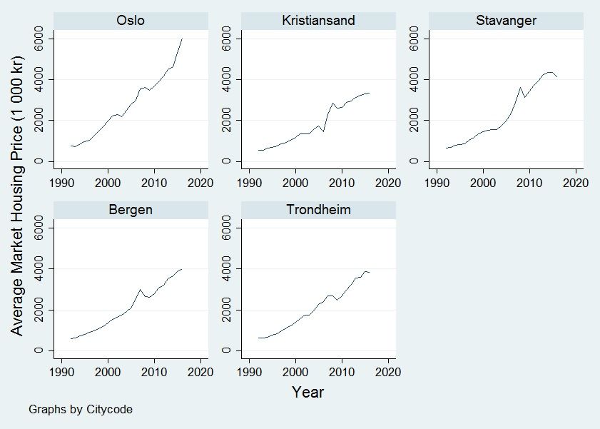
Our housing price data is based on the sum of houses sold and the total value of houses sold. This
gives us the average market housing price in each city. The data includes data for houses, town-
houses, detached, semi-detached and apartments. The composition of the housing types vary over
time so that the data does not illustrate the price development of specific types of housing. Prop-
erties without a stated purchasing price are not included. Analysing the data, we see that Norway
1
Norwegian National Rail Administration were responsible for operating and maintaining the Norwegian railway
network from 1.12.1996 to 31.12.2016, before the agency was divided into The Norwegian Railway Directorate and
Bane NOR
19CHAPTER 4. DATA 20
is no exception to the rising housing market seen elsewhere in the Nordic countries during the last
couple of decades, (Norges Bank (2016)). Figure 4.1 shows the development in housing prices for
our dataset. As expected, the global financial crisis which had most financial assets plummet, also
had a significant impact on housing prices for all cities in our dataset. The years following the
financial crisis had a continuous rise in housing prices with the exception of Trondheim in 2016
and Stavanger in 2015 and 2016. The most astounding development has been in the Capital Oslo,
especially from 2011 to present.
In Stavanger, housing prices dropped by almost 6 percent from 2014-2016, after an average in-
crease of over 8 percent per annum since 2010. This must be seen in light of the development in oil
prices during this period. The price on one barrel of Brent Crude oil dropped by around 35 percent
in 2014 from 109 USD to 70, before adjusting for currency depreciation(Norges Bank (2014)). Ac-
cording to the county-level national accounts for 2014, the oil and gas industry including services,
contributed to one fifth of Rogaland’s gross production at the time of the fall in the oil price.
Figure 4.1: Development in Housing Prices 1992-2016CHAPTER 4. DATA 21
Table 4.1 shows the average housing price for three sub-periods of our dataset. Oslo has the
highest price level in all three periods, followed by Stavanger. In the years 2009-2016 the average
price for housing in Oslo was almost 4.6 million NOK, significantly higher than all the other cities.
Table 4.1: Housing Prices
Average Housing Prices
Oslo Kristiansand Stavanger Bergen Trondheim
1992-1999 1.09 MNOK 0.75 MNOK 0.91 MNOK 0.85 MNOK 0.85 MNOK
2000-2008 2.58 MNOK 1.68 MNOK 2.08 MNOK 2.05 MNOK 2.05 MNOK
2009-2016 4.59 MNOK 3.01 MNOK 3.92 MNOK 3.34 MNOK 3.28 MNOK
4.2 Gross Income
Figure 4.2 shows the development in average per capita gross income in Norwegian Kroner for the
population over 17 years of age. The data is reported in the annual income tax returns. The data
available for 2016 is incomplete and not on municipality levels. Gross Income for 2016 is therefore
estimated based on the average annual growth rate the past five years for each municipality2 . Gross
income includes labour income, trade income, pensions and capital income. Stavanger stands out
as the highest earning municipality in the dataset followed by Oslo and Bergen. The data ranges
from 1993 to 2016, and the five cities have had an average nominal gross income growth of 4.85
percent per annum in this period.
The large decline in gross income in 2006 is due to a change in the tax laws. From 2006, there
were assessed taxes on dividends received for personal tax payers. Previous years this was tax-
free. In 2005, dividends received amounted to NOK 99.3 billion, and in 2006 dividends received
amounted to NOK 7.4 billion3 .
2
The estimation formula is showed in Appendix
3
See Melby (2007)CHAPTER 4. DATA 22
Figure 4.2: Gross Income
All five cities lie above the national average for the entirety of our dataset. In 2015 the average
per capita gross income was 25.8 percent higher in Oslo compared to the national average. Kris-
tiansand, Stavanger, Bergen and Trondheim had an average gross income of 6.6, 37.9, 15.4 and 9.7
percent higher than the national average respectively.
Table 4.2 shows average gross income per capita for three sub-periods of our dataset. Oslo is
the highest earning municipality for the two first sub-periods, while Stavanger is the highest earning
municipality from 2009 to 2016. Kristiansand is the lowest earning municipality in all periods.
Table 4.2: Average Gross Income
Average Gross Income p.c.
Oslo Kristiansand Stavanger Bergen Trondheim
1993-2000 229175 NOK 187750 NOK 220812 NOK 198562 NOK 191375 NOK
2001-2008 349900 NOK 287862 NOK 345150 NOK 304887 NOK 291900 NOK
2009-2016 451190 NOK 390651 NOK 503354 NOK 419693 NOK 399531 NOKCHAPTER 4. DATA 23
Higher gross income per capita attracts residents to the city and increases aggregate demand for
housing. We expect income to have a positive effect on housing prices.
4.3 Unemployment Rate
The unemployment rate is measured as the yearly average of total unemployed persons in per-
centage of the total labor force. The numbers are based on people that register themselves as
unemployed through NAV. There are three criteria in international standards to be registered as
unemployed4 :
• People without income
• People that are searching for work
• People that are available for work
In addition to these criterias, NAV requires that the unemployed person also searches for a job
through NAV. Our dataset consists of people in the ages of 18-74. Figure 4.3 illustrates the de-
velopment in the unemployment rates in our five respective municipalities. All our selected mu-
nicipalities has had the same trend, but with individual differences among percentage rates. The
exeption is the Stavanger region in year 2014 and 2015.
4
See Norwegian Welfare Administration (2017)CHAPTER 4. DATA 24
Figure 4.3: Development in Unemployment Rate 1999-2016
Sørbø and Handal (2010) argues that the unemployment rate increased in affect of the declining
business cycle in the beginning of the millennium. The unemployment continued to increase from
2001 to 2003/04, while declining towards the financial crisis in 2008. The financial crisis had an
impact on the unemployment rate, in the form of higher unemployment. An economy stimulated by
high oil prices and high investments gave a low unemployment rate from 2010 to 2012. Later, the oil
price declined, which has resulted in strong unemployment growth in areas with close connections
to the oil related industry, such as the Stavanger region. The average unemployment rate for Oslo is
3.36 percent for the whole period. Kristiansand, Stavanger, Bergen and Trondheim has an average
of 3.38, 3.00, 2.95 and 3.10 respectively. Table 4.3 shows the average unemployment rate in percent
for our five municipalities, in three sub-periods.CHAPTER 4. DATA 25
Table 4.3: Unemployment Rate
Average Unemployment Rate (%)
Oslo Kristiansand Stavanger Bergen Trondheim
1996-2002 3.3 3.4 3.2 3.5 3.7
2003-2009 3.7 3.2 2.9 3.1 3.5
2010-2016 3.4 3.4 2.6 2.6 2.6
Higher unemployment is often correlated with lower demand in the housing market. In times
of high unemployment, people would often be unsure about their future and be more careful with
their investments. We expect the unemployment rate to have a negative effect on aggregate housing
demand and housing prices.
4.4 Generalised Time Cost of Commuting
In this analysis we have calculated a variable for the generalised time cost of commuting by train in
Norway. The variable is based on the time costs of different components of the travel. The variable
does not include data for the ticket price as ticket prices varies with the same rate across entities
and is accounted for in a fixed effects analysis by the same means as inflation. We therefore use the
term generalised time cost and not generalised cost of commuting.
The dataset is based on timetables for every railway line in Norway from 1997 to 2016, pro-
vided by the Norwegian State Railways. Generating a variable from raw timetables is tedious and
painstaking work, and because this variable will be unique for this thesis, we will dedicate a signif-
icant part of this section to explain the process. The appendix includes specific examples and more
detailed explanation of the process of constructing the generalised time cost variable and its differ-
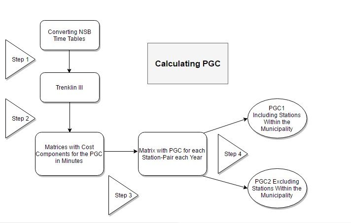
ent components. The flow chart below describes the steps in the process of making the generalised
time cost variable.CHAPTER 4. DATA 26
Figure 4.4: PGC Flow Chart
4.4.1 Converting NSB Time Tables
The first step in the process of making the generalised time cost variable was to convert time
tables, obtained as PDF files from NSB, to a special Microsoft Excel format. The table below
shows the format. The excerpt is from the railway line between Porsgrunn and Notodden called
”Bratsbergbanen” in the Telemark county of Norway. The train stations along the railway line
appears in the first column while the numbers represents the time point of departure and arrival at
each station.CHAPTER 4. DATA 27
Table 4.4: Timetable Entries
Porsgrunn x x
Porsgrunn x 0633
Skien x 0645
Skien 0530 0646
Nisterud 0539 0655
Nisterud 0539 0655
Nordagutu 0559 0721
Nordagutu 0606 0722
Trykkerud 0616 0731
Trykkerud 0616 0731
Notodden 0625 0740
Notodden x x
The stations along a railway line is entered twice along the rows to capture arrival and departure
time at each station. This is to measure eventual time barriers along the trip. The first station on a
railway line would only have a departure time, while the last station on a line would only have an
arrival time. The x symbolises no arrival or departure. As the table shows, the train leaves Skien
at 0530 and arrives the last station Notodden at 0625. In the case of the station Nordagutu in the
second column, the train arrives at 0559 and leaves at 0606. This means 7 minutes of waiting time
on Nordagutu. These 7 minutes is a direct time cost for the traveller, and enters into the persons
generalised time costs of travelling. The third coloumn shows the next departure on the line. The
train now leaves the city of Porsgrunn at 0633, and arrives Notodden at 0740, with a 1 minute break
at both Skien and Nordagutu station. Departures in the weekend and on holidays are not included
in the dataset because of non relevans to commuters. The process of converting PDF time tables to
excel spreadsheets was repeated for every line in Norway from the year 1997 to 2016.
4.4.2 Trenklin III
The Excel spreadsheets with every departure and arrival was ran trough a model made by the Nor-
wegian Railway Directorate called Trenklin III. In Trenklin, generalised time costs are calculated
between all station pairs in Norway based on the route plans that are added to the model and rep-
resents the train service. Ranheim (2017) describes in detail how Trenklin III is created and how it
works. The structure of Trenklin, as applied in our thesis, is the following:
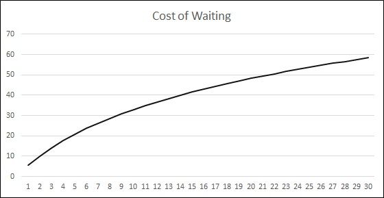
1. In-data and assumptions entered in to-and-from matricesCHAPTER 4. DATA 28 2. Train service in route-plan format added to the model 3. Trenklin III uses algorithms to calculate travel cost components The cost components used to calculate the generalised time cost variable in our thesis are the cost of waiting time at the station, the cost of on board time, the time cost of train transfers and the cost of waiting time related to each transfer. Each of these components are described in detail in the appendix and are included in the total generalised time cost function. An important feature of Trenklin III is that the weights for waiting time is an increasing and diminishing function of the amount of minutes spent waiting. A one minute longer waiting time at the station has less impact on generalised time cost if the waiting time is already high than if the waiting time is short. Trenklin operates with three different travelling purposes; work, leisure and business. These three have different weights for the different components of generalised time cost and different day- distributions of the relevant travelling times. For the purpose of our hypothesis, a special version of Trenklin III has been applied with the generous help of one of our supervisors, Patrick Ranheim, at The Norwegian Railway Directorate. In this version the generalised time cost is calculated using a special day-distribution in which only times relevant for work-related commuting is applied. The day-distribution describes travellers’ preferred arrival time in discrete units, with a value for every minute within 24 hours(i.e a total of 60*24=1440 minutes). This means that the generalised time cost calculations in our thesis are foremost weighted in the periods people travel to and from work. The special day-distribution for our thesis is illustrated in figure 4.5:
CHAPTER 4. DATA 29
Figure 4.5: Day-distribution of Travels Used in Thesis
Source: Norwegian Railway Directorate
The minutes are along the x-axis and the weight for each minute on the y-axis. The weights
sum to 1 over all the minutes within the 1440 minutes. This means that the first peak captures
commuting to work and the second peak captures commuting from work. Commuting to work starts
approximately at 0600 a.m (365/60) and lasts until approximately 1000 a.m(625/60). The period
for commuting from work starts at approximately 1300 p.m(781/60) and lasts until approximately
1900 p.m(1145/60).
The generalised time costs estimates are presented in form of to-and-from matrices for each
year. An example from one of the matrices is presented in the appendix. The matrices shows the
generalised time cost of travelling between each individual station in Norway in minutes.
4.4.3 Calculating The Average Generalised Time Cost for Each City
After the generalised time costs matrices were obtained for each year(1997-2016), stations of rel-
evance for our chosen municipalities were selected. In order to refine stations of relevance to
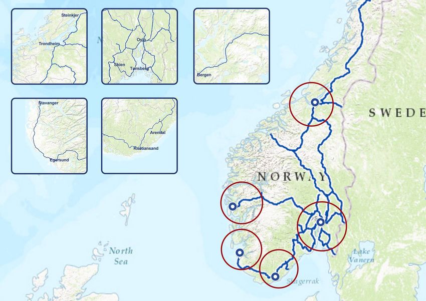
commuting, a radius of 150 minutes of travelling from areas around the municipality in to the cen-
tral station was implemented. We implemented the same radius as Engebretsen et al. (2012) uses
in their report ”Langpendling innenfor intercitytriangelet” on commuting flows within the intercity
triangle in Oslo. Based on this commuting limit, each city’s commuting area is illustrated in the
picture below:CHAPTER 4. DATA 30
Figure 4.6: Central Municipalities and Commuting Radiuses
Map:Bane NOR (Customised by Tora Uhrn)
Since the characteristics of the journey is different depending on which way the journey is,
the generalised time cost is also different. To take this into account, the generalised time costs of
travelling to and from each station of interest was summed together. The average generalised time
costs from the total number of stations within the 150 minutes radius was then calculated.
The next step was to exclude all stations within each municipality. Our analysis uses housing
price data on municipality level. We analyse the effects of a change in the supply of train services
and implicitly the population change. Failure to exclude stations within the municipality would
lead to contradicting effects in housing prices related to improvements in generalised time costs.
Improvements of the railway quality (i.e. a reduction in the generalised time cost) within the
municipality would make living in the municipality more attractive and thereby increase aggregate
demand. We therefore base the generalised time cost variable on travelling to the municipalities’
central station from stations outside the municipalities’ border, but within the commuting limit ofCHAPTER 4. DATA 31
150 minutes. The separation gives two separate variables of the generalised time cost. PGC1 is the
generalised time cost variable for all stations within 150 minutes to the central station and PGC2
is generalised time cost where stations inside the municipality border are excluded. Based on this
rationale, PGC1 should have a smaller and less significant effect on the municipalities’ housing
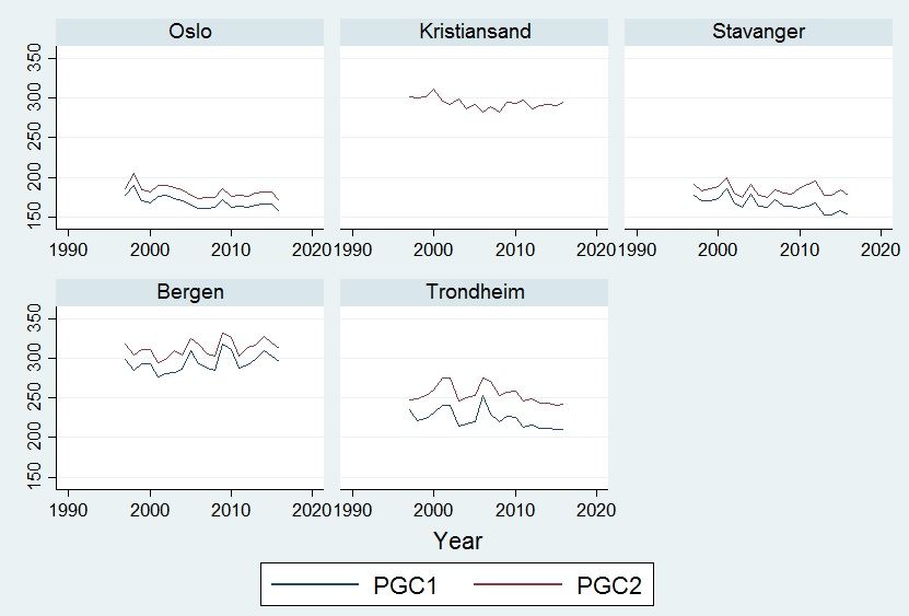
prices. Figure 4.7 shows the development of the PGC variables for both within and outside the
municipality:
Figure 4.7: PGC
Oslo and Stavanger has the lowest average PGC1 and PGC2 for the entire period. All cities
have a lower PGC in 2016 than in 1997 implying an improvement of the railway quality during
our time period in all municipalities. The reduction in generalised time cost is due to changes
in the underlying parameters of the PGC variable. For example, the average on board time has
been reduced from 54.7 minutes in 1998 and 57.7 minutes in 1999 to 52 minutes in 2016, when
travelling by train to Oslo from close by areas. Also, the average amount of train transfers whenCHAPTER 4. DATA 32
travelling into Stavanger has been reduced from 0.60 transfers in 1997, to 0.007 transfers in 2016.
Both examples underlines improvements in railway quality during our time period. The variation
in PGC1 and PGC2 is lowest in Kristiansand, while highest in Trondheim. PGC2 lies above PGC1
in all cities implying that the average generalised time costs is higher when excluding the stations
within the municipality border. The only exception is Kristiansand where no stations other than the
central station lies within the municipality border so PGC1 equals PGC2. The descriptive statistics
for PGC1 and PGC2 within each city is detailed in table 4.5 and 4.6:
Table 4.5: Descriptive Statistics PGC2(minutes)
N Std. deviation Mean Min Max 2016-1997
Oslo 20 7.8 182 170.58 205.33 -14.71
Kristiansand 20 7.10 293.67 282.18 311.80 -6.5
Stavanger 20 7.17 184 174.30 199.62 -14
Bergen 20 10.22 312.63 294.21 331.99 -4.72
Trondheim 20 11.3 254.64 240.42 275.35 -5.24
Table 4.6: Descriptive Statistics PGC1(minutes)
N Std. deviation Mean Min Max 2016-1997
Oslo 20 7.74 168.46 156.83 189.51 -21.17
Kristiansand 20 7.10 293.67 282.18 311.80 -6.5
Stavanger 20 8.85 166.15 152.23 185.56 -24.35
Bergen 20 11.10 294 276.57 317.25 -2.81
Trondheim 20 11.8 223.5 209.69 253.21 -24.44
Oslo has had the biggest improvement in the generalised time cost variable excluding stations
within the municipalities since 1997. Including stations within the municipalities in PGC1, Trond-
heim has had the biggest reduction since 1997. The largest variation is also found in Trondheim.
Based on our hypothesis and the theory of Brueckner(1987), we expect both our generalised
time cost variables to have a positive effect on housing prices, but that the effect of PGC1 to be
smaller than PGC2. This implies an inverse relationship between railway transport quality to and
from the municipality and housing prices within the municipality.CHAPTER 4. DATA 33
4.5 Descriptive Statistics
In this chapter we have presented and described our data with extra attention to the generalised
time cost variable. Table 4.7 summarises the number of observations, global mean values, standard
deviation, minimum value and maximum value for all our variables.
Table 4.7: Descriptive Statistics
Variable Obs Mean Std. Dev. Min Max
Hp 125 2.198 MNOK 1.241 MNOK 0.535 MNOK 6.035 MNOK
unem 105 3.2 % 0.9 % 1.1 % 5.1 %
Y 120 318112 NOK 104207 NOK 154900 NOK 576534 NOK
PGC2 100 247.16 Min 56.17 Min 170.59 Min 332 Min
PGC1 100 229.17 Min 57.72 Min 152.23 Min 317.25 Min
Average housing price is almost 2.2 million NOK with the maximum of 6 million NOK found
in Oslo in 2016. The average unemployment rate over the period 1996 to 2016 for all our munici-
palities is 3.2 percent. Average income from 1992 to 2016 is about 318000 NOK. PGC2 is higher
than PGC1, meaning that generalised time costs of commuting is higher when excluding stations
within the municipalities.
In the next chapter we will present and discuss our baseline model. We also discuss relevant is-
sues regarding panel data analysis. We will present a static model as well as a dynamic specification
which allows for sluggish adjustments in housing prices.You can also read