Postural Orthostatic Tachycardia Syndrome explained using a baroreflex response model
←
→
Page content transcription
If your browser does not render page correctly, please read the page content below
Postural Orthostatic Tachycardia Syndrome explained using a
                                                                    baroreflex response model
                                                                              Justen Geddes1 , Johnny T Ottesen2 ,
                                                                             Jesper Mehlsen3 and Mette S. Olufsen1
arXiv:2109.14558v1 [q-bio.TO] 27 Sep 2021

                                                                                        September 30, 2021

                                                                                               Abstract
                                                       Recent studies have shown that Postural Orthostatic Tachycardia Syndrome (POTS) patients
                                                   have abnormal low frequency ≈ 0.1 Hz blood pressure and heart rate dynamics. These dynamics
                                                   are attributed to the baroreflex and can give insight into the mechanistic causes which are the
                                                   basis for proposed subgroups of POTS. In this study we develop a baroreflex model replicating the
                                                   low-frequency dynamics observed in POTS patient data as well as represent subgroups of POTS
                                                   in our model. We utilize signal processing to quantify the effects that model parameters have
                                                   on low-frequency oscillations. Results show that key physiological parameters that represent the
                                                   hypothesized causes are central to our model’s ability to reproduce observed dynamics from patient
                                                   data.
                                            1   Department of Mathematics North Carolina State University, Raleigh, NC, 27695, USA
                                            2   Department of Science and Environment, Roskilde University, Denmark
                                            3   Section for Surgical Pathophysiology, Rigshospitalet, Denmark

                                            1      Introduction
                                            Postural Orthostatic Tachycardia Syndrome (POTS) is characterized by the presence of tachycardia upon
                                            the transition to an upright position in addition to a history of persistent (at least six months) symptoms,
                                            absence of orthostatic hypotension, and absence of other condition provoking sinus tachycardia [15, 17,
                                            37]. Symptoms include mild to severe brain fog, palpitations, visual blurring, and/or dizziness. Since
                                            POTS is a phenotype and not a specific disease, it is difficult to identify the compromised mechanisms.
                                            This is partly due to POTS’ numerous potential causes, including dehydration, neuropathy, or the
                                            presence of agonistic antibodies binding to specific adrenergic receptors [32, 37]. POTS is typically
                                            diagnosed by examining heart rate and blood pressure in response to a postural challenge, such as head-
                                            up tilt (HUT) or active standing [51]. These signals are measured continuously and re-ported along
                                            with a description of symptoms, yet diagnosis primarily relies on a single quantity - tachycardia (heart
                                            rate increase > 30 bpm, > 40 bpm for adolescents) [51, 53].
                                                Reliance on postural tachycardia to diagnose POTS is problematic as the single measure does not
                                            provide insight into the mechanistic causes underlying the syndrome. Recent studies [18, 56, 42], have
                                            observed that not only do POTS patients exhibit tachycardia, increasing heart rate higher than normal
                                            in response to postural change, they also experience increased 0.1 Hz heart rate and blood pressure
                                            oscillations. Curently, clinical diagnosis only includes one POTS group, but as suggested by Mar, Raj, and
                                            Fedorowski [37, 15], POTS may have three phenotypes: (1) neuropathic POTS caused by neuropathy in
                                            the vascular beds, particularly in the lower body; (2) hypovolemic POTS attributed to low fluid volume
                                            in the body and (3) hyperadrenergic POTS characterized by high levels of circulating norepinephrine

                                                                                                   1
during postural change inducing an exaggerated sympathetic response (Grubb08). Diagnosis of these
subtypes typically involves multiple tests as phenotypes can be challenging to identify from heart rate
and blood pressure response to a single HUT test.
     It is known that POTS patients typically experience compromised baroreflex function [37, 18].
Several hypotheses have been put forward suggesting what parts of the system are compromised, though
it is difficult to determine how each factor impacts dynamics. As a result, most patients receive a series
of tests to examine their dynamic response. This study uses a mathematical model to investigate how
the system responds when parameters associated with each phenotype are varied. More insight into how
the system reacts to a specific change may reduce the number of tests needed for accurate diagnosis.
     For healthy people, the baroreflex system operates via negative feedback modulating sympathetic
and parasympathetic nerve activity mitigating blood pressure changes. Stretch receptors in the aortic
arch and carotid sinus detect changes in blood pressure modulating firing rate in the afferent vagal nerve,
which sends signals to the nucleus tractus solitarius (NTS). From here, the signals are transmitted via
the efferent sympathetic and parasympathetic nerves. Heart rate is modulated by changes in the firing of
both sympathetic and parasympathetic nerves, while the sympathetic nervous system primarily modulates
the peripheral vascular resistance and cardiac contractility. At rest, sympathetic activity is low (≈ 20%
of its maximum), while the parasympathetic activity is high (≈ 80% of its maximum) [28]. In response
to a decrease in blood pressure, the afferent signaling is inhibited, leading to parasympathetic withdrawal
and sympathetic stimulation increasing in heart rate, cardiac contractility, and peripheral resistance [3].
Numerous studies have examined baroreflex signaling [9, 11, 42], and it has been established that blood
pressure and heart rate are controlled by negative feedback with a resonance frequency of approximately
0.1 Hz. This response is easily distinguished from heart rate with a frequency of 1 Hz and respiration,
which oscillates with a frequency of 0.2 − 0.3 Hz [11].
     As noted earlier, several recent studies have examined the magnitude, and phase of the low frequency
≈ 0.1 Hz) blood pressure and heart rate oscillations in POTS patients [18, 42, 56]. The studies by
Stewart et al. [56] and Medow et al. [42] used Transcranial Doppler measurements of cerebral blood
flow and finger arterial plethysmography to analyze blood flow and heart rate oscillations in response to
a postural challenge. Using auto-spectral and transfer function analysis, they reported that increased
low-frequency oscillations in arterial pressure led to increased oscillations in cerebral blood flow, which
they suggest may be responsible for the “brain fog” experienced by many POTS patients. These results
agree with our findings using empirical mode decomposition to examine blood pressure and heart rate
signals measured during HUT from females diagnosed with POTS. We found that the magnitude of the
0.1 Hz heart rate (HR) and blood pressure (BP) oscillation was increased during HUT and that the
instantaneous phase difference between low-frequency HR and BP signals is shorter in POTS patients
than in control subjects, at rest and during HUT [18]. These studies indicate that POTS patients have
compromised baroreflex and that it is likely that both the sympathetic and parasympathetic branches
are compromised. Several studies [6, 15, 37] discuss what parts of the system may be compromised,
but it is difficult to obtain direct measures explaining how specific pathophysiology impact heart rate
and blood pressure dynamics.
     One way to gain more insight into how a specific pathophysiology impacts the system dynamics is
by building mechanistic models and comparing signals from controls and POTS patients. Numerous
studies have examined the baroreflex feedback dating back to studies by Bronk and Stella [5] and by
Landgren et al. [30] who built a mechanical apparatus to study how changes in pressure modulate the
firing of the baroreceptor nerves in the carotid artery in rabbits and cats. Data were analyzed using a
simple mathematical model. This study was followed by a series of studies [54, 2, 20, 55] using modeling
to relate blood pressure and heart rate. The study by Mahdi et al. [35] gives an overview of several early
models. The most notable results are by Beneken and DeWitt, who modeled the baroreflex as a transfer
relation with two “regions” - the first associating large changes in pressure with a short time-constant,

                                                    2
and the second smaller changes in pressure with a larger time-constant, and the comprehensive model
by Guyton [20] explaining blood pressure control. Since then, numerous researchers have examined
various aspects of the baroreflex system, including several contributions by Ursino et al. (e.g., [57, 58])
describing the principal baroreflex mechanisms. These early studies focused on describing mechanisms
underlying the baroreflex function, while the more recent studies focus on calibrating models to data. An
example is the study by Bugenhagen et al. [7] that used blood pressure as an input to fit spontaneous
baroreflex regulation of heart rate in salt-sensitive Dahl rats.
These models must be translated to examine the response to typical postural challenges such as HUT
and active standing imposed to understand human pathophysiology. Several studies have examined the
response to orthostatic stress challenges, e.g., [23, 45, 14, 27, 49, 63, 40]. For example, the model by
Olufsen et al. [46] used heart rate as an input to predict the blood pressure response to active standing.
The model demonstrates that model predictions can match a healthy young adult’s blood pressure
by estimating patient-specific cardiovascular parameters modulating peripheral vascular resistance and
vascular compliance. In [63] this approach was adapted to study the response to HUT. In Matzuka et
al. [40] parameter estimation was carried using Kalman Filtering, while the study by Williams et al. [62]
and Matzuka et al. [40] used optimal control theory to estimate model parameters.
While these studies all captured variations in response to a postural change, none tested the frequency
of baroreflex changes examining the power of the characteristic 0.1 Hz oscillations. To our knowledge,
only a few studies have attempted to test if dynamical systems models dis-play 0.1 Hz oscillations. The
study by Heldt et al. [24] built a model predicting low-frequency oscillations in astronauts undergoing
a sit-to-stand test using a baroreflex control model. They found that the low-frequency oscillations
emerging from their model did not persist after the transition from sit-to-stand. Another attempt was
made by Hammer and Saul [21], who used an open loop baroreflex model to predict the response to a
postural change. This model uses arterial blood pressure as an input to predict heart rate. While this
model examines the 0.1 Hz oscillations, it does not study how the response changes in time; instead,
it quantifies stability at fixed operating points responsible for low-frequency oscillations. More recently,
Ishbulatov et al. [25] use a closed-loop baroreflex model to replicate low-frequency aspects of patient
data during a passive HUT test. This study analyzes how a healthy human body adapts to an orthostatic
challenge. However, this model is complex and does not study the response in POTS patients.
To remedy the shortcomings of these previous studies, we use a simple closed-loop differential
equations model without delays to examine temporal and frequency baroreflex response to HUT for
POTS patients.
To our knowledge, no previous studies have combined a mechanistic model with signal analysis to
explain the emergence and modulation of the low-frequency oscillations for POTS patients. To do so,
we develop a systems-level baroreflex model to explain the low-frequency dynamics observed in POTS
patients both at rest and during HUT. We use simulations to display how the three POTS phenotypes
identified by [37] can be encoded in the model and how these possibly affect blood pressure and heart
rate dynamics. Our model is formulated using a simple closed-loop 0D cardiovascular model, with
basic first-order control equations representing the baroreflex regulation. We analyze our model using
signal processing techniques and study the effects of critical model parameters that correspond to the
physiological abnormalities that cause each POTS phenotype. Results indicate that changes in clinically
relevant parameters can result in the emergence of low-frequency oscillations with amplitude equal to
that observed in POTS patient data from our previous study [18]. Discussion of our results focuses on
clinical implications and motivation of future studies.
32 Methods
This study develops a closed-loop 0D model describing the emergence of low-frequency (≈ 0.1 Hz)
oscillations observed in POTS patients. The model is parameterized to match average blood pressure
and heart rate signals measured during HUT. Simulation results are depicted with characteristic POTS
data. The model is simulated both at rest and during HUT with varying parameters that differentiate
the three phenotypes suggested by Mar and Raj [37].
Similar to previous studies [63, 48], we predict blood flow and pressure in the systemic circulation
using an electrical circuit model with five compartments, including the upper and lower body arteries and
veins, and the left heart (see Figure 1Aii). The baroreflex is incorporated via negative feedback control-
equations predicting the effector response (heart rate, vascular resistance, and cardiac contractility) as
functions of mean arterial pressure (Figure 1Ai). The magnitude and phase of the low-frequency oscil-
lations generated by the baroreflex are extracted using discrete Fourier transform, analyzing computed
heart rate and blood pressure signals.
Computations are first conducted in the supine position, followed by HUT simulated by shifting
blood from the upper to the lower body. We demonstrate the importance of incorporating heart rate
variability by adding uniformly distributed noise to predictions of heart rate, and discuss how phenotypes
suggested by Mar and Raj can be simulated.
2.1 Data
The model simulations are qualitative in nature and meant to illustrate how changing system properties
impact dynamics. But test if the outcome of our simulations make sense in terms of physiological
behavior, we included blood pressure and heart rate measurements (extracted from [18]) from two
representative subjects: a control and a POTS patient.
Measurements from these people include continuous ECG and upper arterial blood pressure mea-
surements extracted at rest for 5 minutes and then for 5 additional minutes after the HUT onset. Heart
rate is extracted from intervals between consecutive RR waves obtained from a 3-lead ECG, and con-
tinuous blood pressure measurements are obtained using a Finapress device (Finapres Medical Systems
BV, Amsterdam, Netherlands). Blood pressure and ECG signals are sampled at 1000 Hz. Heart rate
is extracted from the high-resolution ECG measurements as the inverse distance between consecutive
RR intervals. Blood pressure and heart rate signals are sub-sampled to 250 Hz, after which the Uni-
form Phase Empirical Mode Decomposition [18] is used to extract the magnitude and phase of 0.1 Hz
oscillations.
The afferent input to the baroreflex control model assumes that blood pressure is measured at the
level at the carotid barorecptors (above the center of gravity). Therefore blood pressure data, measured
at the level of the heart, is adjusted by subtracting the effect of gravity as described in our previous
study [63].
2.2 Cardiovascular model
We employ an electrical circuit analogy to predict blood flow (analogous to current), pressure (anal-
ogous to voltage), and volume (analogous to charge) in the systemic circulation represented by five
compartments, including the upper (u) and lower (l) body arteries (a) and veins (v), and the left heart
(lh). Each compartment is quantified by its volume (V (t) ml) and pressure (P (t) mmHg), while flow
Q(t) (ml/s) exists between compartments. Figure 1 depicts the model and Table 1 lists the dependent
cardiovascular variables.
4(B)0.76
(A)
H (bps)
0.73
(i) BR
120
P (mmHg)
100
80
Left
Left Heart
Ventricle
400 450 500
(lh)
(lv)
Time (s)
(mv) (av)
(C)
B HR Power Spectrum
Amplitude (mmHg) Amplitude (bps)
Upper
(ii) Upper body
BR
RSA body
0.01
Veins Nod Arteries
(vu) e (au)
0.005
0
(v) Lower
(up) body (a)
Pressure Power Spectrum
Lower 10
Lower body body
Veins Arteries 5
(vl) (al)
0
0.2 0.4 0.6 0.8 1
Frequency (Hz)
(lp)
Figure 1: (Ai) Hemodynamics is controlled by the baroreflex system, which senses changes in the upper
body arteries (lumping thoracic and carotid baroreceptors). Afferent signals from baroreceptor neurons
are integrated into the brain and transmitted via sympathetic and parasympathetic neurons regulating
heart rate, peripheral vascular resistance, and left heart elastance. (Aii) The systemic circulation is
represented by compartments lumping upper (au) and lower (al) body arteries, upper (vu) and lower
(vl) body veins, and the left heart (lh). Flow (Q) through the aortic valve (av) is transported from the
left heart to the upper body arteries. From here, it is transported in the arteries (a) to the lower body
arteries and through the upper body peripheral vasculature (up) to the upper body veins. A parallel
connection transports flow through the lower body peripheral vasculature (lp). From the lower body
venous flow (v) is transported to the upper body veins and finally via the mitral valve (mv) back to
the left heart. Each compartment representing the heart or a collection of arteries or veins has pressure
(P ), volume (V ), and elastance (E). Pumping of the heart is achieved by assuming that left heart
elastance (Elh (t)) is time-varying. (B) Model predictions of heart rate (H (bps), top panel) and upper
body arterial pressure (Pau (mmHg), lower panel). The blue line shows pulsatile blood pressure and the
red the mean pressure (Pm ). 5-second sections of each signal are shown in the overlaid subpanels. (C)
Frequency spectra of time-series data (H top, Pau bottom) shown in (B).
To ensure flow conservation, for each compartment (i = lh, au, al, vl, vu), the change in volume is
computed as the difference between flow into and out of the compartment,
dVi
= Qin − Qout , (1)
dt
5where Qin denotes the flow into, and Qout denotes the flow out, of compartment i. Ohm’s law relates
flow to pressure and the resistance (R, mmHg s/ml) between compartments (i − 1) and (i),
Pi−1 − Pi
Qi = . (2)
Ri
For each arterial compartment and upper venous compartment i, pressure and volume are related using
the linear relation
Pi − Pui = Ei (Vi − Vui ), (3)
where Vui is the unstressed volume, Ei is the elastance (reciprocal of compliance, analogous to capaci-
tance), and Pui = 0 is the unstressed pressure.
Given that pressure changes significantly on the venous side, in particular in the lower venous
compartment during HUT, as suggested by Hardy et al. [22] we employ a nonlinear relation between
lower venous pressure and volume given by
1 V
M vl
Pvl = log (4)
mvl VM vl − Vvl
where mvl is a parameter that relates nominal pressure, volume (Vvl ) and maximal volume (VM vl ) [50].
The pumping of the heart is achieved by introducing a time-varying elastance function of the form
ES −ED πt
2
1 − cos( TS ) + ED 0 ≤ t ≤ TS
Elh (t) = ES −E cos π(t−T S)
2
D
TD + 1 + ED TS ≤ t ≤ TS + TD (5)
ED TS + TD ≤ t ≤ T,
where ES , ED , TS , and TD denote the end systolic and end diastolic elastance, the time for systole and
diastole, respectively.
The timing parameters TS and TD are determined as functions of the length of the previous cardiac
cycle (the RR interval). By combining the prediction of the length of the QT interval from [1, 29] and
the ratio of cardiac mechanical contraction to relaxation from [26], we get
c2 c2
TS = 0.45 c1 + , TD = 0.55 c1 + , (6)
RR RR
where c1 = 0.52 s and c2 = −0.11 s2 from [1].
Similar to arterial compartments, the left heart pressure Plh and volume Vlh are related by
Plh − Plh,u = Elh (t)(Vlh − Vun ), (7)
where Plh,u = 0 and Vlh,u = 10 are the unstressed pressure and volume in the left heart, and Elh (t) is
the time-varying elastance.
2.3 Head-up tilt (HUT)
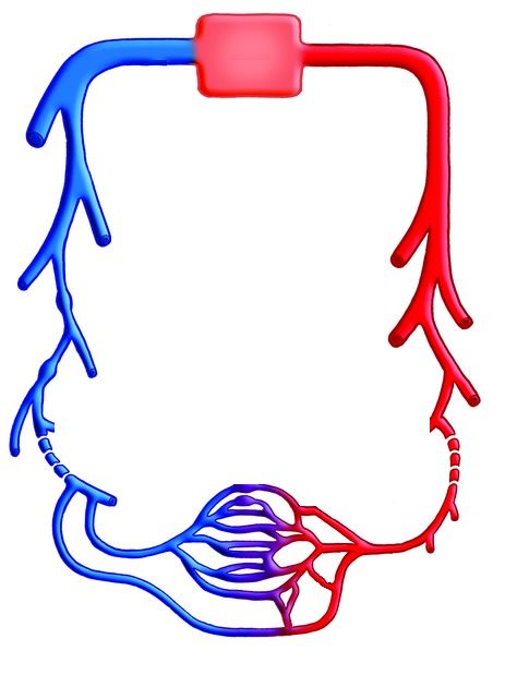
During HUT, gravity pools blood from the upper to the lower body affecting the flow between the upper
and lower body (Qa and Qv ). This maneuver is depicted in figure 2. We model this effect by adding a
tilt term accounting for the additional force caused by gravitational pooling [63], i.e.
Pau − Pal + Ptilt Pvu − Pvl − Ptilt
Qa = , Qv = , (8)
Ra Rv
where θπ
Ptilt = ρgh sin , θ ∈ [0◦ , . . . , 60◦ ]. (9)
180
6Table 1: Dependent variables (volume V (ml), pressure P (mmHg), and flow Q (ml/s) ) for the
cardiovascular system and baroreflex control system. The latter includes peripheral vascular resistance
Rup and Rlp , left ventricular elastance Elv , and heart rate H.
State variables
Symbol Description States Units
R Resistance Upper peripheral (up) mmHg · s/ml
Lower peripheral (lp) mmHg · s/ml
E Elastance Left heart (lh) mmHg/ml
Diastolic value of left ventricle elastance (ED) mmHg/ml
P Pressure Left heart (lh) mmHg
Arteries, upper (au) mmHg
Arteries, lower (al) mmHg
Veins, upper (vu) mmHg
Veins, lower (vl) mmHg
Mean (m) mmHg
V Volume Left heart (lh) ml
Arteries, upper (au) ml
Arteries, lower (al) ml
Veins, upper (vu) ml
Veins, lower (vl) ml
Q Flow Atrial valve (av) ml/s
Arteries (a) ml/s
Upper peripheral (up) ml/s
Lower peripheral (lp) ml/s
Veins (v) ml/s
Mitral valve (mv) ml/s
H Heart rate - bps
Figure 2: Depiction of a head-up tilt (HUT) test. Patients are tilted, head up, from 0 to 60◦ over of 7
seconds.
2.4 Baroreflex model
The baroreflex (BR) control system maintains homeostasis. Afferent baroreceptor nerves sense changes
in the aortic arch and carotid sinus blood pressure (both are included in the compartment represent-
ing the upper body arteries). Signaling in afferent baroreceptor neurons stimulated by blood pressure
are integrated into the medulla, from which efferent neurons are activated, modulating signaling along
7sympathetic and parasympathetic neurons. In the systemic circulation, parasympathetic neurons mainly
modulate heart rate, while sympathetic neurons modulate cardiac contractility, peripheral vascular re-
sistance, and vascular elastance.
This study includes a simple model directly modulating effector sites in response to changes in blood
pressure. Equations for the effector variables X = {Rup , Rlp , Em , H} (listed with units in Table 2)
are derived under the assumption that each response has a saturation point and a resting value. This
assumption motivates the use of first-order kinetic control equations given by
dX −X + X̃(P̄ )
= , (10)
dt τX
where τX is the time-constant for the response X (shorter for effectors stimulated via parasympathetic
than via sympathetic neurons). P̄ denotes the average BP, computed as
dP̄ −P̄ + Pau
= (11)
dt τP
and X̃ is an increasing or decreasing Hill function of the form
P̄ kX
X̃ = (XM − Xm ) kX
+ Xm (12)
P̄ kX + P2X
or
kX
P2X
X̃ = (XM − Xm ) kX
+ Xm (13)
P̄ kX + P2X
where XM is the maximum value of X̃, Xm is the minimum, P2X is the half-saturation value, and kX
is the Hill coefficient. Graphs of increasing and decreasing Hill functions, with varying kX are shown in
Figure 3.
Table 2: Quantities controlled by the Baroreflex system using Hill functions. Columns correspond to the
quantity being controlled, the symbol of control equation, whether the hill function used is increasing
or decreasing, and units.
Quantity being controlled Symbol Increasing/Decreasing Units
Resistance, upper peripheral R̃up Decreasing mmHg · s/ml
Resistance, lower peripheral R̃lp Decreasing mmHg · s/ml
Elastance at end diastole ẼD Increasing mmHg/ml
Heart Rate H̃ Decreasing bps
2.5 Heart rate variability (HRV)
In addition to changes in blood pressure mediated by the baroreflex control system, heart rate data
exhibit spontaneous variation, referred to as heart rate variability [36]. This is likely due to fluctuations
in vagal firing and has proven to be essential for cardiovascular dynamics. While it is well established
that HRV is associated with fluctuations in vagal firing setting up a mechanistic model predicting HRV
is challenging. To circumvent this, several studies have referred to HRV as mathematical chaos [19,
52]. This study examines the importance of including HRV, which we model by adding “noise” to heart
rate predictions.
8Increasing Hill Function Decreasing Hill Function
kX =4
XM kX =8
kX =12
kX =16
kX =4
kX =8
kX =12
Xm
kX =16
P2X P2X
Figure 3: Increasing and decreasing Hill functions for varying Hill-coefficients kX .
We solve the differential equations one cycle at a time, and use current heart rate to determine the
length of the next cycle T = 1/H. HRV is obtained by adding noise to each cardiac cycle sampled from
a uniform distribution, i.e., we let
1 U[−1, 1]
T ← · 1+ , (14)
tH0 H tH0
50
where U[−1, 1] is a uniform random distribution from -1 to 1, and tH0 denotes the starting time for
each heartbeat. We choose to scale the noise by 2% to approximately match patient data.
2.6 Model parameters and initial conditions
Nominal parameter values and initial conditions are deduced from literature and physiological data
representing a healthy young female. Below we describe a priori calculation of the parameters, which
are listed with units in table 3. This Table include values used to simulate both control and POTS
phenotypes.
2.6.1 Cardiovascular parameters
Blood volume: Blood volume is calculated using height and Body Mass Index (BMI). Combining the
h 2
classic formula for BMI [60] by which weight is given by W = BMI 100 , with Nadler’s equation for
blood volume (BV) [43],to estimate female blood volume (ml) as
BV = 0.4948 BMI0.425 h1.575 − 1954
and male blood volume (ml) as
BV = 0.4709 BMI0.425 h1.575 − 1229
where h is height in cm. For our baseline patient we use the average height of women in Denmark,
167.2 cm [10], and a “healthy” BMI of 22 kg/m2 [60].
9The total blood volume (BV) is distributed between the systemic (containing ≈85%) and pulmonary
(containing ≈15%) circulations [3]. Within the systemic circulation, at rest, we assume that approxi-
mately 15% is in the arteries and 85% is in the veins. In the supine position, we assume that 80% of
the blood is in the upper body, while only 20% is in the lower body [3]. To predict circulating blood
volume, we differentiate the volume between stressed (circulating) and unstressed volume. Following
Beneken and DeWitt [2], in the arteries, we assume that 30% of the volume is stressed, while in the
veins we assume that 7.5% of the total volume is stressed.
Blood pressure: The model is parameterized to represent dynamics in a healthy young female with a
systolic arterial pressure of 120 mmHg and diastolic arterial pressure of 80 mmHg [31]. Using standard
clinical index [12], we compute the mean pressure as Pm = (2/3) · Pdia + (1/3) · Psys ≈ 93 [41]. As
blood pressure is typically measured in the arm, which is included in the upper body arteries, we assign
these values to the upper arterial compartment. To allow for blood flow from the upper to the lower
body arteries, we set the lower body artery pressure to 0.98 times values in the upper body. Since the
venous circulation’s pulse-pressure is small, we only determine mean values in venous compartments.
Using standard literature values [3] we assume that the upper body venous pressure is 3 mmHg, again
to ensure flow in the correct direction, the lower body venous pressure is Pvl = 1.1 · Pvu .
Parameters for the lower body venous pressure-volume equation (equation 4) are calculated as
VM vl = 4 · VvlI
1 VM vl
mvl = log
PvlI VM vl − VvlI
where VvlI , PvlI and VM vl is the nominal volume, pressure and maximal volume for the lower venous
compartment (vl) respectively. VM vl is set such that the volume does not saturate at HUT, and mvl is
set such that at rest, blood flows from the lower to the upper body veins.
Elastance: To calculate nominal Elastance values, we use equation 3. Assuming that Pun = 0 and
the stressed volume fractions discussed above, we predict elastance for arterial compartments and the
upper veins. Due to our use of a non-linear venous pressure-volume equation (equation 4), we do not
calculate lower venous elastance explicitly. To capture effect of changing the pulse-pressure during HUT
this parameter is adjusted following the HUT onset.
Left heart end-diastolic and end-systolic elastance: At the end of diastole, the pressure of the left heart
is approximately equal to the venous pressure, and the ventricular volume is maximal, i.e., the nominal
(minimal) elastance at diastole can be approximated by
ED = Pvu / max(Vlh ). (15)
Similarly, at the end of systole, the left ventricular pressure is approximately equal to the arterial pressure,
and the volume is minimal, giving the nominal (maximal) elastance at systole
ES = Pau / min(Vlh ). (16)
Blood flows: In a healthy human cardiac output (CO) is approximately 5 L/min [3]. We assume that
the total blood volume is circulated in approximately 60 seconds, i.e., the cardiac output CO≈ BV /60
ml/s. We assume that all organs above the pelvis, including the gastrointestinal tract, belong to the
upper body, while the lower pelvic region and the legs belong to the lower body. With this distinction,
we estimate that 80% of cardiac output travels through the upper peripheral, perfusing the upper
body, while 20% perfuse the lower body [61]. Hence we obtain nominal values of Qup = 0.8CO, and
Qa = Qlp = Qv = 0.2CO.
10Resistance: The atrial and mitral valve resistance are both set to 0.0001, as we assume the valves
do not have significant resistance compared to resistance generated by flow through the vasculature.
Therefore, the remaining nominal resistances are calculated using Ohm’s law, R = (Pi−1 −Pi )/Q, where
Pi−1 is the pressure in the previous compartment, Pi is the pressure in the destination compartment,
and Q is the flow.
2.6.2 Baroreflex control parameters
Each control equation has 4 parameters, τX , XM , Xm , and P2X . The time-constant, τX , reflects the
ratio of the speed of the neurological responses and time for the physiological control to occur. We
note that the parasympathetic branch (τH ) operates faster than the sympathetic (τR , τE ), i.e.,
τH < τR = τE
Following our calculation of the base parameters, at rest, we assume that controlled parameters are at
equilibrium, i.e., at P = P0 , dX
dt = 0. Using this assumption, we can estimate P2X as
X
M− X0
P2X = P0 , X = ED ,
X0 − Xm
X −X
0 m
P2X = P0 , X = Rup , Rlp , H.
XM − X0
The maximum heart rate (HM ) is set to 3.3 bps [44], and we assume a minimum heart rate of Hm = 0.3
bps, representing the smallest sustainable heart rate possible in humans. We allow peripheral vasculature
to dilate to 1.5 times the resting radius and constrict to 0.75 times the resting radius. To relate these
measurements to changes in resistance we note that resistance changes in proportion to the fourth power
of the radius. Thus we assume that Rm = 0.2 · RI and RM = 3 · RI .
To estimate EDM , we refer to the increased potassium levels, which increases cardiac contractility,
that has been recorded during exercise in humans [34]. From this work, we estimate the extent to which
contractility can increase under stress and assume that maximum end-diastolic elastance control (EDM )
can increase to 125% of the initial value. In principle, the heart can relax completely by lack of stimulus.
We therefore set the minimum end-diastolic elastance control (EDm ) to 1% of the initial value.
2.6.3 Initial conditions
Initially, we set the phase of the heart to the end of diastole. Thus VlvI = 110 − Vun , where 110 is the
maximum volume of the left ventricle, and Vun is the unstressed volume of the left ventricle, which we
assume to be 10 ml [8]. We also assume a physiologically healthy resting initial heart rate of 1 bps.
The remaining initial conditions are set to the calculated nominal values.
2.7 Signal processing
To characterize oscillations seen in the model output, we employ stationary signal processing. This
process is illustrated in Figure 4. Once the model has been simulated using MATLAB’s [39] ode15s
and there are no transient effects, we interpolate over the data to obtain a time-series that is sampled
uniformly at 100 Hz. We then select the last 200 seconds of the H and Pau time-series and compute
the one-sided power spectrum using MATLAB’s FFT algorithm. The design of our model suggests two
explainable oscillations: one representing the baroreflex, which operates at approximately 0.1 Hz, and the
heart rate, which operates at approximately 1 Hz. As can be seen in Figure 4 these two oscillations and
their harmonics are the only significant spikes in the frequency domain. To quantify the magnitude of
11Table 3: Table of parameters, their descriptions, values, and units. The character “X” represents the
control quantities that can be found in table 2. Unit abbreviations are: mmHg - millimeters of mercury,
s - seconds, ml - milliliters, bps - beats per second, N.D. - no dimension, ED - end diastole, ES - end
systole, coef. - coefficient. The cardiovascular parameters were the same for all phenotypes simulated,
while the control parameters differ. Table 2 lists values used for each phenotype.
Symbol Description Value Units Ref
h Height 167.2 cm [10]
BMI Body mass index 22 kg/m2 [60]
BV Total blood volume 3887.9 ml [13, 43]
Vun Unstressed volume 10 ml [8]
Rav Aortic valve resistance 0.0001 mmHg s/mmHg
Rmv Mitral valve resistance 0.0001 mmHg s/mmHg
Ra Resistance of systemic arteries 0.072 mmHg s/mmHg [38]
Rv Resistance of systemic veins 0.019 mmHg s/mmHg [38]
Eal Elastance lower body arteries 3.1 ml/mmHg [3]
TS Time-fraction for maximum systole 0.12 s [1, 26, 29]
TD Time-fraction for minimum diastole 0.14 s [1, 26, 29]
EES ES ventricular elastance 2 mmHg/ml Equation 16
kR Resistance Hill coef. 23 N.D.
kE Diastolic ventricular elastance Hill coef. 7 N.D.
kH Heart rate Hill coef. 27 N.D.
τR Resistance time-constant 12.5 s
τE ED ventricular elastance time-constant 12.5 s
τR Heart rate time-constant 6.25 s
τP Mean arterial pressure time-constant 2.5 s
XM Maximum value controlled effector
Xm Minimum value controlled effector
P2X Half-saturation coef. (pressure) mmHg
oscillations caused by our control equations, we record the power and phase of the maximum amplitude
peak in the ≈ 0.1 Hz frequency range. This process is applied both for the model at rest and computed
again for the HUT portion.
2.8 Emergence of low-frequency oscillations
To capture the emergence of low-frequency ≈0.1 Hz oscillations we first conducted a parameter sweep
changing all relevant parameters over their physiological range. Specific emphasis is on parameters
in equations facilitating baroreflex control (Equations 10-13). This analysis is done in two steps, first
detecting what parameters impact the dynamic behavior and second conducting a detailed analysis
varying critical parameters impacting the dynamic response. In addition, to detecting what parameters
cause the model to change behavior, we also investigate how to set parameters to capture oscillations
at the ≈ 0.1Hz frequency range.
Pseudo-code for this analysis is included in Table 4. The model is solved initially for 250 seconds.
After 250 seconds the solution is examined to verify that the solution has reached steady state for 200
seconds. To verify steady state behavior the previous 200 seconds are split in half and maximum and
minimum heart rate (H) and upper arterial blood pressure (Pau ) are calculated for each half and the
12Figure 4: Process of obtaining amplitude of the 0.1 Hz component of a heart rate signal, the same
process is used for blood pressure. Starting from the left, first the simulation is ran using a variable
step size solver and is interpolated at 100 Hz. The last 200 seconds are recorded (darkened portion).
Second, the discrete Fourier transform is applied to obtain amplitude information of the frequencies.
We select and examine the range corresponding to the baroreflex, 0.05 - 0.15 Hz (darkened). Third, we
find the maximum of the amplitude in this range (darkened).
relative difference between values for each half is computed and compared to a threshold (α). The
halves are then interpolated at 100 Hz and Fourier power spectra are computed for heart rate and blood
pressure for each half. The maximum ≈ 0.1 Hz power value is recorded for each half and the relative
difference between the power of the halves are computed and compared to a threshold (β). If all of
these relative differences are less than their respective thresholds the model is said to be a steady state
and the power spectra of the last 200 seconds is computed and recorded. If at least one of the relative
differences is above the threshold the model is solved for 20 additional seconds and checked for steady
state behaviour again.
This approach allows for an automated way to explore the parameter space. Doing so we can
observe Hopf bifurcations with respect to the low-frequency oscillations and can observe the effects of
parameters on the strength of oscillations.
13Two-dimensional parameter analysis pseudo-code
Input: Parameter values
Output: Amplitude and frequency of ≈ 0.1 Hz response, H & Pau
α ← 0.01
β ← 0.1
T2 ← 250
While: t ≤ T2
Run model for one heartbeat, tH ← t+ duration of heartbeat
IF: tH ≥ T2
T0 ← T2 − 200
T1 ← T 0+T
2
2
max H([T0 ,T1 ]) −max H([T1 ,T2 ])
C1 ← ≤α
max H([T1 ,T2 ])
min H([T0 ,T1 ]) −min H([T1 ,T2 ])
C2 ← ≤α
min H([T1 ,T2 ])
max Pau ([T0 ,T1 ]) −max Pau ([T1 ,T2 ])
C3 ← ≤α
max Pau ([T1 ,T2 ])
min Pau ([T0 ,T1 ]) −min Pau ([T1 ,T2 ])
C4 ← ≤α
min Pau ([T1 ,T2 ])
Interpolate H,Pau at 100 Hz to obtain H̃,P̃au
Compute AH1 , AH2 , AP 1 , AP 2
IF: AH2 > 0
C5 ← AH1A−AH2
H2
≤β
ELSEIF: AH1 == AH2 , C5 ← 1
ELSE: C5 ← 0
END
IF: AP 2 > 0
1 −AP 2
C6 ← A P A P2
≤β
ELSEIF: AP 1 == AP 2 , C6 ← 1
ELSE: C6 ← 0
END
IF: min(C1 , C2 , C3 , C4 , C5 , C6 ) == 0
T2 ← T2 + 20
END
END
t ← tH
END
Calculate and record metrics
END CODE
Table 4: Pseudo code for two-dimensional parameter analysis. H([Ti , Tk ]) represents the value of heart
rate (H) between time of Ti and Tk , similarly for blood pressure Pau . AH1 denotes the amplitude of
the 0.1 Hz component of the H signal during [T0 , T1 ] as is explained in methods section 2.7. Similarly,
AP 1 for Pau . AH2 and AP 2 are denote the amplitude of the approximately 0.1 Hz component during
[T1 , T2 ]. Analysis is conducted for both rest and head-up tilt sections.
142.9 POTS and its phenotypes
We model POTS and its phenotypes suggested by [37] by adjusting parameters to reflect the hypothe-
sised physiology. The values of the parameters before and after HUT can be seen in Table 5.
The hyperadrenergic POTS is characterized by high levels of circulating norepinephrine during pos-
tural change, which allows the sympathetic nervous system to be more responsive to changes in blood
pressure. To simulate this, at the onset of HUT we further increase parameters associated with sympa-
thetic response including P2H and kH , kE , kR .
Neuropathic POTS is caused by partial neuropathy of the lower body vasculature, which causes
abnormal pooling of blood in the lower extremities. To simulate this, we decrease the control for the
lower body resistance by reducing RlbM and Rlbm after HUT.
The hypovolemic POTS is obtained by decreasing the total blood volume. In isolation, this phenotype
does not compromise the baroreflex, and should therefore not be specified as an individual phenotype.
However, we do acknowledge that a large number of patients with severe POTS side-effects are young
skinny females. However, rather than modeling low blood volume as a phenotype we investigate how
the two phenotypes are represented in normotensive and hypervolumic individuals.
To allow for a smooth transition between parameter values that allows for a 10-second delay, we
translate the change in parameters mimicking incorporating a delayed onset, i.e.;
(
x0 t < tHU T + 10
x= (t−tHU T −10)8 (17)
(x1 − x0 ) (t−tHU T −10)8 +58 + x0 t ≥ tHU T + 10
where x is the parameter being changed after HUT, x0 is the value of the parameter during rest, x1 is
the value of the parameter that is being transitioned to and tHU T is the time of the start of the HUT.
Phenotype Parameter Value before tilt Value after tilt
Control Cau 1.15 ml/mmHg 0.69 ml/mmHg
P2H 89 mmHg 87 mmHg
Hyperadrenergic kH 27 N.D. 47 N.D.
kR 23 N.D. 40 N.D.
kE 7 N.D. 12 N.D.
P2H 88.7 mmHg 89.6 mmHg
Cau 1.15 ml/mmHg 0.69 ml/mmHg
Neuropathic RlpM 4.5 mmHg · s/ml 2.9 mmHg · s/ml
Rlpm 0.30 mmHg · s/ml 0.19 mmHg · s/ml
Cau 1.15 ml/mmHg 0.69 ml/mmHg
Table 5: Values of selected parameters before and after head-up tilt for phenotype simulations. Pa-
rameters are as follows: Cau - upper arterial compliance, P2H - half saturation value for heart rate
control, kH - Hill coefficient for heart rate control, kR - Hill coefficient for resistance control, kE - Hill
coefficient for left heart end diastolic elastance control, RlpM - maximum value of resistance control,
Rlpm - minimum value of resistance control.
3 Results
Results demonstrate the emergence of low-frequency oscillations at rest and during HUT and how the
phenotypes proposed by Mar and Raj [37] can be simulated.
153.1 Low-frequency oscillations
Our model, shown in Figure 1, can generate ≈0.1 Hz heart rate (H) and blood pressure (Pau ) oscillations
observed in patient data [18]. The amplitude and frequency of the oscillations can be modulated by
varying the model parameters in the baroreflex control equations (Equations 10-13), including the
maximum XM and minimum Xm response, the time-constants τX , the half-saturation values P2X , and
the Hill-coefficients kX , X = H, R, E.
Oscillation frequency is primarily determined by time-constants (τX ) differentiating the parasym-
pathetic and sympathetic control. Efferent responses mediated by the parasympathetic system are
significantly faster than those transmitted via the sympathetic system [3], i.e., τH
τR = τE . The
0.1 Hz frequency was achieved using time-constants reported in Table 3. We observe that the Hill
coefficients (kX ) also have an effect on frequency but to a lesser extent than τX .
Oscillation amplitude can be modulated by changing kX , P2X and XM − Xm , X = H, R, E. We
studied the effect of varying all parameters over their physiological range. Results (summarized in
Table 6) show that kX , X = H, R, E impact the oscillation amplitude, with kH being more influential.
Increasing the Hill-coefficients kX increases the sensitivity of the baroreflex control. A larger value of kX
gives a steeper set-point function (shown in Figure 3), i.e., the change in pressure needed to generate
a given response decreases. Shifting the Hill function by changing the half saturation value (P2X ) can
cause the operating regime to change to a steeper portion of the Hill function. This shift causes has
the same effect as increasing kX but has a much smaller effect on oscillation amplitude.
Figure 5A (top panels) shows HR and BP dynamics in response to increasing kH . We depict results
changing kH as the most influential parameter, but similar results (not shown) are obtained when
increasing kR and kE , controlled by the sympathetic system. For kH < 6, the system does not oscillate,
at kH ≈ 6, oscillations emerge, and their amplitude increases with increasing values of kH . Figure
5B depicts the change in amplitude and frequency as a function of kH . Changing kX , X = H, R, E
impacts the oscillation amplitude more than frequency. The frequency almost doubles (it changes from
0.6Hz to 1.1 Hz) while the HR oscillation amplitude increases from ≈0 to 0.3. The frequency diagrams
in Figure 5B (right column) have two characteristic features, a broad distribution (vertical spread) and
horizontal stripes with white spacing. The former results from noise, added to heart rate, to account
for heart rate variability, and the latter by the frequency resolution. The model is solved with a time
step of 0.01 s, with the Fourier transform calculated over a 200 s interval, giving a frequency resolution
of 0.005 Hz.
As noted above, kH has the most significant impact on the system dynamics. Both the sympathetic
and parasympathetic systems control heart rate, but as noted in the introduction, POTS may be the
result of the expression of specific agonistic antibodies binding to β1 and β2 receptors [37]. Since these
are found on pacemaker cell modulating heart rate and smooth muscle cells in the vasculature, we study
the response to changing kH and kR . Results shown in Figures 6A and 6B reveal that increasing either
kH or kR increases the amplitude of oscillations. This result agrees with the hypothesis that POTS
patients have a more sensitive control system.
The other model parameters also change the dynamic behavior - but not as significant as changes in
kX (specifically kH ). In general, the half-saturation value offsets the control at different pressure levels
but does not change the sensitivity, as the slope of the sigmoidal curve remains the same. Changing
the range ∆X = XM − Xm changes the width and steepness of the curve; the latter does have some
effect on sensitivity, but it is not as significant as the effect observed when increasing kX . Table 6 lists
the effects of changing each parameter on HR and BP.
16Increased Parameter Effect
kH Increases H & Pau oscillation amplitude
kR Increases H & Pau oscillation amplitude
kE Increases H & Pau oscillation amplitude
P2H Increases H, increases diastolic Pau
P2R Decreases H, increases Pau
P2E Decreases H, increases H & Pau oscillation amplitude
Increases Pau pulse-pressure
HM − Hm Increases H & Pau oscillation amplitude
RM − Rm Increases H & Pau oscillation amplitude
EDM − EDm Increases H & Pau oscillation amplitude
Table 6: Effects on heart rate (H) and upper arterial blood pressure (Pau ) when increasing stated
parameter.
3.2 Head-up tilt (HUT)
During HUT (shown in Figure 2), gravity pools blood from the upper to the lower body, stimulating
the autonomic nervous system. The result is a shift in blood volume and pressure, increasing in com-
partments below the center of gravity and decreasing in compartments above. In our model, the upper
body compartments are centered around the carotid baroreceptors, while the lower body compartments
are centered in the lower part of the torso. Representative model blood pressure predictions in all com-
partments are shown in Figure 8. We note that after HUT, the pressure in the lower compartments
increases while pressure in the upper compartments decreases. These simulations were generated with
kH = 27, which causes the system to oscillate at rest and after HUT. Without changing parameters,
oscillations dampen after HUT as a result of volume redistribution.
Similar to rest, control parameters impact predicted dynamics, and kH remains the most influential
parameter. Figures 6A (bottom row) shows oscillation amplitude as a function of kR and kH without
noise. For these simulations, the ”non-oscillatory” region appears striped, indicating bands of oscillations
alternating with no oscillations. Figure 6C shows selected time-series predictions for parameter values
marked on Figure 6A. We note that in the non-oscillatory region, it is possible to increase kH and
eliminate oscillations. These stripes are a result of the on-off behavior of emerging low-frequency
oscillations. Mathematically, this behavior is common; as we change kR or kH the system undergoes
repeated Hopf bifurcations. However, physiologically, small changes in a parameter have not been
reported to affect the frequency response significantly. By adding noise mimicking heart rate variability
(HRV) to the model, this behavior disappears (the striped pattern disappears, see Figure 6B), suggesting
that the presence of HRV stabilizes the system response as can be seen in Figures 6B and 6D.
3.3 POTS phenotypes
Previous studies [37, 15] suggest that POTS patients can be separated into neuropathic, hyperadrenergic,
and hypovolemic phenotypes. This section discusses how each of these can be represented in our model.
Note, we do not have blood pressure or heart rate data annotated with specific phenotypes. Therefore
the results presented here depict qualitative rather than quantitative.
The phenotype encoding is based on the assumption that the cardiovascular system of POTS patients
changes in response to a postural change. For this reason, select parameters change after HUT in order
to recreate dynamics observed in data. We select which parameters to change based on the phenotype
that we are representing. We decrease the upper body arterial compliance for all simulations to account
17kH = 10 kH = 20 kH = 30
1.1 1.1 1.1
H (bps)
1 1 1
0.9 0.9 0.9
120 120 120
Pau (mmHg)
100 100 100
80 80 80
60 60 60
600 650 700 600 650 700 600 650 700
Time (s) Time (s) Time (s)
Max. and Min. ~0.1 Hz Osc Amp Frequency of Osc
1.4 0.3 0.12
H Frequency (Hz)
0.1
H (bps)
1.2 0.2
0.08
1 0.1
0.06
0.8 0
10 20 30 40 10 20 30 40 10 20 30 40
Pau Frequency (Hz)
0.12
120 10
Pau (mmHg)
0.1
100
5 0.08
80
0.06
60 0
10 20 30 40 10 20 30 40 10 20 30 40
kH kH kH
Figure 5: (A) From left to right: heart rate (H, top) and upper arterial pressure (Pau , bottom) predictions
for kH = 10, 20, and 30. (B) From left to right: maximum and minimum values of predictions for varying
values of kH , the amplitude of the 0.1 Hz region response, and frequency of oscillations. Enlarged red
dotes show denote measurements corresponding to kH = 10, 20, 30.
for the redistribution of volume upon HUT. The values of the changed parameters before and after HUT
can be seen in Table 5
Control subjects show a limited increase in heart rate and similar amplitudes of oscillations before
and after HUT. When volume is redistributed during HUT, the baroreflex control operating regime is
shifted due to upper arterial pressure decreasing. To avoid an increase in heart rate, we shift the heart
rate response curve with the pressure by decreasing P2H . Simulation of a control subject can be seen
18Amp ~0.1 Hz H (bps) Amp ~0.1 Hz P au (mmHg) Amp ~0.1 Hz H (bps) Amp ~0.1 Hz P au (mmHg)
30 0.025 1.8 30 0.025 1.8
kR - Rest
kR - Rest
40 PH PH 40 PH PH
CR CR CR CR
50 50
60 0 0 60 0 0
5 10 15 20 25 5 10 15 20 25 5 10 15 20 25 5 10 15 20 25
40 0.025 1.8 40 0.025 1.8
50 50
kR - HUT
kR - HUT
PH PH PH PH
60 CR 60 CR
CR CR
70 70
0 0 0 0
50 60 70 50 60 70 50 60 70 50 60 70
kH kH kH kH
(a) kR vs kH (b) kR vs kH with 2% noise.
(4) H (bps) (3) H (bps) (2) H (bps) (1) H (bps)
1.52
(4) H (bps) (3) H (bps) (2) H (bps) (1) H (bps)
1.5
1.45 1.47
1.4 1.42
1.5 1.52
1.45 1.47
1.4 1.42
1.57 1.58
1.52 1.53
1.47 1.48
1.59 1.59
1.54 1.54
1.49 1.49
220 230 240 250 260 270 280 220 230 240 250 260 270 280
Time (s) Time (s)
(c) HUT time-series for 4 red dots marked (d) HUT time-series for 4 red dots marked
in sub-figure 6a in sub-figure 6b
Figure 6: Two-dimensional parameter analysis of kR vs. kH . (A) Amplitudes of peak heart rate (H)
oscillation (left) and peak upper arterial blood pressure (Pau ) oscillation (right) at the ≈ 0.1 Hz frequency
band for values of kR and kH at rest (top) and head-up tilt (HUT, bottom). (B) The same information
as (A) but with 2 % noise. Average measurements from data [18] are marked for Control patients at rest
(CR), and POTS patients during head-up tilt (PH). Note that the physiologically possible oscillations
correspond to the green regions. (C) Heart rate predictions during HUT for red dots on lower panels of
(A); ith panel from top corresponds to ith dot from the left in (A). (D) Similar information as (C) but
pertaining to (B).
with data in the left column of 9.
Hyperadrenergic POTS patients have increased levels of plasma norepinephrine during HUT [37].
We model this by increasing ki , i = H, E, R and P2H during HUT. Results, depicted in Figure 9 (top row
center), show that increasing these parameters increases the amplitude of 0.1 Hz oscillations (compared
to the control subject - top left) and causes tachycardia during HUT, which is consistent with POTS
patient data.
19Amp ~0.1 Hz H (bps) Amp ~0.1 Hz P au (mmHg) Amp ~0.1 Hz H (bps) Amp ~0.1 Hz P au (mmHg)
2000 0.025 1.8 2000 0.025 1.8
3000 3000
BV - Rest
BV - Rest
PH PH PH PH
4000 4000
CR CR CR CR
5000 5000
6000 0 0 6000 0 0
15 20 25 30 35 15 20 25 30 35 15 20 25 30 35 15 20 25 30 35
2000 0.025 1.8 2000 0.025 1.8
BV - HUT
BV - HUT
2500 PH PH 2500 PH PH
CR CR CR CR
3000 3000
3500 0 0 3500 0 0
40 50 60 70 40 50 60 70 40 50 60 70 40 50 60 70
kH kH kH kH
(a) BV vs kH (b) BV vs kH with 2% noise.
Figure 7: Two-dimensional parameter analysis of blood volume (BV) vs kH . (A) Amplitudes of peak
heart rate (H) oscillation (left) and peak upper arterial blood pressure (Pau ) oscillation (right) at the
≈ 0.1 Hz frequency band for values of BV and kH at rest (top) and head-up tilt (HUT, bottom). (B)
The same information as (A) but with 2 % noise. Average measurements from data [18] are marked for
Control patients at rest (CR), and POTS patients during head-up tilt (PH).
1.5
100
Plv
H
50
1 0
140
120
120
Pau
100
Pal
100
80 80
60 60
4
20
3
Pvu
Pvl
10
2
0
950 1000 1050 950 1000 1050
Time (s) Time (s)
Figure 8: Results of simulation with HUT at t = 1000. Row 1: heart rate, H (bps), left ventricle
pressure, Plv (mmHg) row 2: upper arterial pressure, Pau (mmHg), lower arterial pressure, Pal (mmHg)
row 3: upper venous pressure, Pvu (mmHg), lower venous pressure, Pvl (mmHg).
Neuropathic POTS patients experience excessive blood pooling below the thorax during HUT due
to partial autonomic neuropathy. This condition is simulated by decreasing the range of resistance
control in the lower body arteries, i.e., we reduce Ralp,M and Ralp,m making this control less effective.
20Results from this simulation depicted in Figure 9 top right show that subjects exhibit tachycardia but
that oscillations are dampened after HUT onset.
Hypovolemia To understand how hypovolemia impacts our predictions, we reduce central blood vol-
ume. We found that hypovolemia alone was not able to reproduce POTS dynamics such as increased
oscillations or tachycardia. We instead study the effects of hypovolemia on the other phenotypes. Re-
sults shown in Figure 9 bottom row show that heart rate is lower compared to patients with a normal
blood volume, but for hyperadrenergic POTS patients, the amplitude of the heart rate and blood pres-
sure oscillations increase significantly, indicating that this patient group may experience more severe
response to POTS. To study this phenomenon further, we conducted a two-dimensional analysis exam-
ining the amplitude of heart rate and blood pressure oscillations as a function of blood volume (BV)
and kH at rest and during HUT.
Figures 7A and 7B (top row) show that reducing blood volume at rest does not impact dynamics.
However, as can be seen in the bottom row of Figures 7A and 7B, reducing blood volume during HUT
increases oscillation amplitude. This implies that more severe oscillations occur during HUT for patients
with less blood volume. Similar to Figure 6, Hopf bifurcation lines can be seen in the parameter space
in Figure 7A but are removed when noise is added to simulations representing heart rate variability as
can be seen in Figure 7B.
Control, BV = 4500 ml Hyperadrenergic, BV = 4500 ml Neuropathic, BV = 4500 ml
1.6 1.6
1.6
1.4 1.4
H (bps)
H (bps)
H (bps)
1.4
1.2 1.2
1.2
1 Data Data
1 Data
Model
1 Model Model
0.8 0.8
120 120 120
Pau (mmHg)
Pau (mmHg)
Pau (mmHg)
100 100 100
80 80 80
60 60 60
940 960 980 1000 1020 1040 1060 940 960 980 1000 1020 1040 1060 940 960 980 1000 1020 1040 1060
Time (s) Time (s) Time (s)
Control, BV = 3500 ml Hyperadrenergic, BV = 3500 ml Neuropathic, BV = 3500 ml
1.6 1.6
1.6
1.4 1.4
H (bps)
H (bps)
H (bps)
1.4
1.2 1.2
1.2
1 Data Data
1 Data
Model
1 Model Model
0.8 0.8
120 120 120
Pau (mmHg)
Pau (mmHg)
Pau (mmHg)
100 100 100
80 80 80
60 60 60
940 960 980 1000 1020 1040 1060 940 960 980 1000 1020 1040 1060 940 960 980 1000 1020 1040 1060
Time (s) Time (s) Time (s)
Figure 9: Characteristic data and model predictions of heart rate (H), upper arterial blood pressure
(Pau ), and mean pressure. Simulations with 4500 ml of blood are in the top row with simulations
with 3500 ml of blood in the bottom row. Cau is decreased after HUT for all simulations to represent
constriction of vasculature upon HUT. In control P2H is decreased (left), kH and P2H are increased
after HUT to replicate hyperadrenergic POTS (middle) and kH increased, RlpM and Rlpm decreased to
replicate neuropathic POTS (right).
214 Discussion
This study developed a closed loop baroreflex cardiovascular model and used simple signal processing to
extract the frequency and amplitude of heart rate and blood pressure oscillations. Results show that our
model can generate oscillations in the low-frequency ≈ 0.1 Hz) range observed in control and POTS
patients at rest and during head-up tilt (HUT) and that oscillations can be manipulated by modulating
parameters associated with the baroreflex.
Our model can predict tachycardia (an increase in HR of at least 30 bpm, 40 bpm in adolescents)
observed in POTS patients by increasing the half-saturation of the heart rate response (P2H ) or de-
creasing the maximum and minimum vascular resistance (RlpM and Rlpm ). The former is significantly
more effective than the latter. Moreover, by changing physiologically relevant baroreflex parameters
after HUT, we can reproduce the hyperadrenergic and neuropathic POTS phenotypes suggested by [15,
37]. Finally, we found that predictions are highly sensitive to changes in blood volume, suggesting that
short skinny patients may experience a more severe reaction than females with a normal blood volume.
4.1 Low-frequency oscillations
The mathematical model used here extends previous studies [11, 24, 63, 38, 40, 38, 57, 59] predicting
cardiovascular dynamics using a closed loop lumped parameter model including the left heart, the upper
and lower body systemic arteries, and veins. The latter is included to facilitate the redistribution of
volume upon postural change. The baroreflex is modeled using a first-order control equation predicting
the controlled quantity as a function of pressure using sigmoidal function enforcing saturation at both
high and low values of the controlled parameter.
By modulating parameters associated with the baroreflex sensitivity (the sigmoidal kX , X = R, E, H,
we explain the emergence and amplification of the low-frequency oscillations at rest and during HUT.
Our findings agree with those reported in our previous study [18], noting that the low-frequency os-
cillations (sometimes referred to as Mayer waves) are observed in all subjects and that the oscillation
amplitude is increased in POTS patients in particular following HUT. Our findings also agree with
previous experimental studies that report larger low-frequency oscillations in cerebral blood flow [42,
56].
While this phenomenon has been discussed in studies using signal processing to examine heart rate
and blood pressure time-series, only a few studies by Ottesen et al. [47] and Ishbulatov et al. [25]
used closed loop modeling to replicate this phenomenon. Both these studies explained the emergence
of oscillations by introducing a delay in sympathetic response. In contrast, our model predicts the
emergence of the ≈ 0.1 Hz oscillatory response without introducing delay differential equations.
These findings agree with the hypothesis that POTS patients may have an abnormally sensitive
baroreflex control. Specifically, we observed that kH is the most influential parameter for the oscillation
amplitude. At kH < kcritical , the system does not oscillate, but as kH increases, oscillations emerge via
a Hopf bifurcation. In addition, we found that the baroreflex time-constants modulate the oscillation
frequency.
To better understand how key physiological parameters modulate oscillation amplitude, we conducted
a 2-dimensional parameter analysis. Figure 6 shows that during rest and HUT, increased peripheral
resistance and heart rate response sensitivities (kR , kH ) increase oscillation amplitude. We see in Figure
6 that during HUT, increased blood volume decreases oscillation. This agrees with clinical insights from
Klinik Mehlsen that patients with smaller blood volume have more pronounced POTS symptoms.
22You can also read