Real Time Head Pose Estimation with Random Regression Forests
←
→
Page content transcription
If your browser does not render page correctly, please read the page content below
Real Time Head Pose Estimation with Random Regression Forests
Gabriele Fanelli1 Juergen Gall1 Luc Van Gool1,2
1 2
BIWI, ETH Zurich ESAT-PSI / IBBT, KU Leuven
{fanelli,gall,vangool}@vision.ee.ethz.ch vangool@esat.kuleuven.be
Abstract
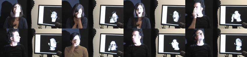
Fast and reliable algorithms for estimating the head pose
are essential for many applications and higher-level face
analysis tasks. We address the problem of head pose esti-
mation from depth data, which can be captured using the
ever more affordable 3D sensing technologies available to-
day. To achieve robustness, we formulate pose estimation
as a regression problem. While detecting specific face parts
like the nose is sensitive to occlusions, learning the regres-
sion on rather generic surface patches requires enormous Figure 1. Real time head pose estimation example.
amount of training data in order to achieve accurate esti-
mates. We propose to use random regression forests for the
task at hand, given their capability to handle large training tion can finally allow us to overcome some of the prob-
datasets. Moreover, we synthesize a great amount of anno- lems inherent of methods based on 2D data. However, ex-
tated training data using a statistical model of the human isting depth-based methods either need manual initializa-
face. In our experiments, we show that our approach can tion, cannot handle large pose variations, or are not real-
handle real data presenting large pose changes, partial oc- time. An exception are approaches like the one presented
clusions, and facial expressions, even though it is trained by [4], where the authors achieve real-time performance by
only on synthetic neutral face data. We have thoroughly exploiting the massive parallel processing power of a GPU.
evaluated our system on a publicly available database on Their approach relies on a geometric descriptor which pro-
which we achieve state-of-the-art performance without hav- vides nose location hypotheses which are then compared
ing to resort to the graphics card. to a large number of renderings of a generic face template,
done in parallel on the GPU. The fast computation time
reported is only achievable provided that specific graphics
1. Introduction
hardware is available.
Automatic and robust algorithms for head pose estima- GPUs, however, present a very high power consump-
tion can be beneficial to many real life applications. Accu- tion which limits their use for certain kinds of application.
rately localizing the head and its orientation is either the ex- Hence, we propose an approach for 3D head pose estima-
plicit goal of systems like human-computer interfaces (e.g., tion which does not rely on specific graphics hardware and
reacting to the user’s head movements), or a necessary pre- which can be tuned to achieve the desired trade-off between
processing step for further analysis, such as identification accuracy and computation cost, which is particularly useful
or facial expression recognition. Due to its relevance and to when resources are limited by the application. We formu-
the challenges posed by the problem, there has been consid- late the problem as a regression, estimating the head pose
erable effort in the computer vision community to develop parameters directly from the depth data. The regression
fast and reliable algorithms for head pose estimation. is implemented within a random forest framework [2, 10],
Methods relying solely on standard 2D images face seri- learning a mapping from simple depth features to a prob-
ous problems, notably illumination changes and textureless abilistic estimation of real-valued parameters such as 3D
face regions. Given the recent development and availabil- nose coordinates and head rotation angles. Since random
ity of 3D sensing technologies, which are becoming ever forests (as any regressor) need to be trained on labeled data
more affordable and reliable, the additional depth informa- and the accuracy depends on the amount of training, data
617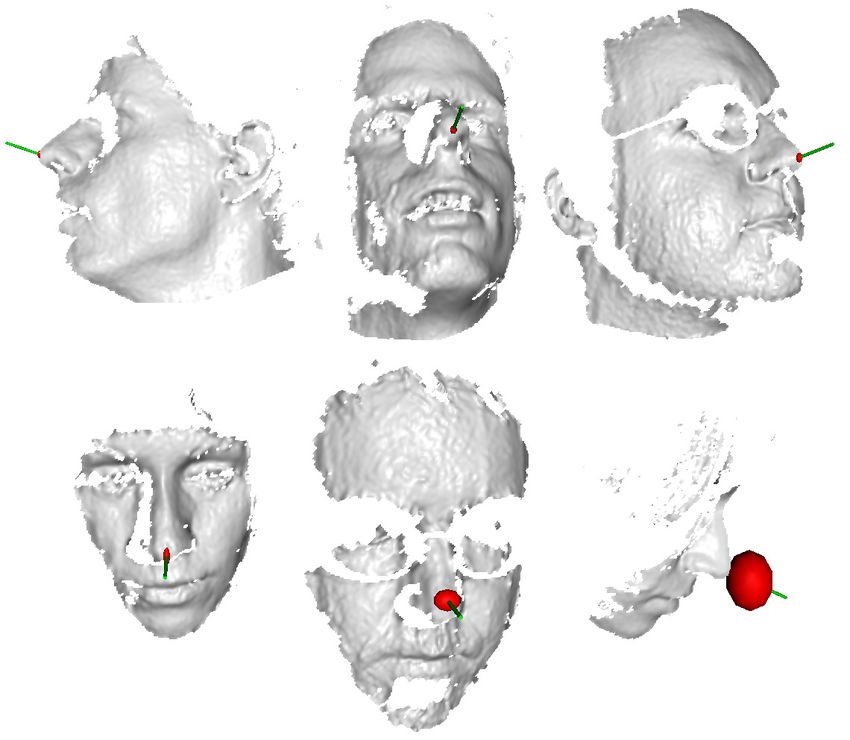
acquisition is a key issue. We solve this problem by train-             images [5, 18, 24]. Seemann et al. [24] presented a neu-
ing only on synthetic data, generating an arbitrary num-                ral network-based system fusing skin color histograms and
ber of training examples without the need of laborious and              depth information. It runs at 10 fps but requires the face
error-prone annotations. Our system works in real-time on a             to be first detected in frontal pose. The work of [5] uses a
frame-by-frame basis, without any manual initialization or              linear deformable face model for real-time tracking of the
expensive calculations. In our experiments, we show that it             head pose and facial movements using depth and appear-
works for unseen faces and can handle large pose changes,               ance cues. Their system focuses on tracking facial features
variations such as facial hair, and partial occlusions, e.g.,           and thus no evaluation is presented for its head pose track-
due to glasses, hands, or missing parts in the 3D reconstruc-           ing performance. The approach presented in [17] uses head
tion. Moreover, as it does not rely on specific features, e.g.,         pose estimation only as a preprocessing step to face recog-
for the nose tip detection, our method can be adapted to the            nition, and the reported errors are only calculated on faces
localization of other parts of the face. The performance of             belonging to the same people. Breitenstein et al. [4] pro-
the system is evaluated on a challenging publicly available             posed a real-time system which can handle large pose vari-
database and our results are comparable or superior to the              ations, partial occlusions (as long as the nose remains visi-
state-of-the-art.                                                       ble), and facial expressions from range images. The method
                                                                        uses geometric features to generate nose candidates which
2. Related Work                                                         suggest many head position hypotheses. Thanks to the mas-
                                                                        sive parallel computation power of the GPU, they can si-
    Head pose estimation is the goal of several works in                multaneously compare all suggested poses to a generic face
the literature [19]. Existing methods can conveniently be               template previously rendered in many different orientations
divided depending on the type of data they rely on, i.e.,               and finally choose the pose minimizing a predefined cost
2D images or depth data. Within the 2D image-based al-                  function. Also the authors of [15] use range images and
gorithms, we can further distinguish between appearance-                rely on the localization of the nose; however, their reported
based and feature-based methods. While the former look                  results are computed on a database generated by syntheti-
at the entire face region in the image, the latter rely on the          cally rotating frontal scans of several subjects.
localization of specific facial feature points.
                                                                           Random forests [2] have become a popular method in
    A common appearance-based approach is to discretize
                                                                        computer vision [11, 10, 20, 14, 12] given their capabil-
the head poses and learn a separate detector for each pose,
                                                                        ity to handle large training datasets, high generalization
e.g., [13, 18]. Approaches like [1, 6] focus on the map-
                                                                        power, fast computation, and ease of implementation. Re-
ping from the high-dimensional space of facial images into
                                                                        cent works showed the power of random forests in mapping
lower-dimensional, smooth manifolds; Osadchy et al. [21],
                                                                        image features to votes in a generalized Hough space [11] or
for example, use a convolutional network, detecting faces
                                                                        to real-valued functions [10, 12]. Recently, multiclass ran-
and their orientation in real-time. Several works rely on
                                                                        dom forests have been proposed in [12] for real-time head
statistical models of the face shape and appearance, e.g.,
                                                                        pose recognition from 2D video data. To the best of our
Active Appearance Models (AAMs) [8] and their exten-
                                                                        knowledge, we present the first approach that uses random
sions [9, 23, 25], but their focus is usually on detection and
                                                                        regression forests for the task of head pose estimation from
tracking of facial features.
                                                                        range data.
    Feature-based methods need either the same facial fea-
tures to be visible in all poses, e.g., [26, 29, 16], or use
pose-dependent features; for example, Yao and Cham [30]                 3. Head Pose Estimation with Random Regres-
select feature points manually and match them to a generic                  sion Forests
wireframe model. The authors of [28] use a combination
                                                                           Our goal is to jointly estimate the 3D coordinates of the
of the face appearance and a set of specific feature points,
                                                                        nose tip and the angles of rotation of a range image of a
which bounds the range of recognizable poses to the ones
                                                                        head, i.e., 2.5D data output of a range scanner like [27].
where both eyes are visible.
                                                                        We use a random regression forest (Sec. 3.1), trained as ex-
    In general, methods relying solely on 2D images are
                                                                        plained in Sec. 3.2 on a large dataset of synthetically gen-
sensitive to illumination, lack of features, and partial oc-
                                                                        erated range images of faces (Sec. 3.4). The way the actual
clusions. Moreover, the annotation of head poses from
                                                                        regression is performed is explained in Sec. 3.3.
2D images is an error-prone task in itself. Fortunately,
recent 3D technologies have achieved high quality at af-
                                                                        3.1. Random Regression Forests
fordable costs, e.g., [27]. The additional depth informa-
tion can help in solving some of the limitations of image-                 Classification and regression trees [3] are powerful tools
based methods, therefore several recent works use depth ei-             capable of mapping complex input spaces into discrete or
ther as primary cue [4, 15] or as an addition to standard 2D            respectively continuous output spaces. A tree achieves

                                                                  618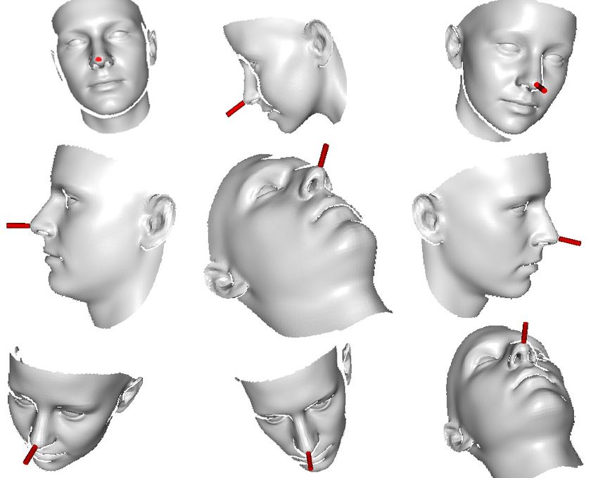
highly non-linear mappings by splitting the original prob-                   over neighboring, non-border pixels. The real-valued vector
lem into smaller ones, solvable with simple predictors.                      θi = {θx , θy , θz , θyaw , θpitch , θroll } contains the pose pa-
Each node in the tree consists of a test, whose result directs               rameters associated to each patch. The components θx , θy ,
a data sample towards the left or the right child. During                    and θz represent an offset vector from the point in the range
training, the tests are chosen in order to group the training                scan falling on the center of the training patch to the nose
data in clusters where simple models achieve good predic-                    position in 3D, while θyaw , θpitch , and θroll are the head
tions. Such models are stored at the leaves, computed from                   rotation angles denoting the head orientation.
the annotated data which reached each leaf at train time.                       We build the trees following the random forest frame-
   Breiman [2] shows that, while standard decision trees                     work [2]. At each non-leaf node, starting from the root,
alone suffer from overfitting, a collection of randomly                      a test is selected from a large, randomly generated set of
trained trees has high generalization power. Random forests                  possible binary tests. The binary test at a non-leaf node is
are thus ensembles of trees trained by introducing random-                   defined as tf,F1 ,F2 ,τ (I):
ness either in the set of examples provided to each tree, in                                  X                          X
the set of tests available for optimization at each node, or in                     |F1 |−1          I f (q) − |F2 |−1          I f (q) > τ,   (1)
both. Figure 2 shows a very simple example of the regres-                                     q∈F1                       q∈F2
sion forest used in this work.
                                                                             where I f indicates the feature channel, F1 and F2 are two
                                                                             rectangles within the patch boundaries, and τ is a threshold.
                                                                             The test splits the training data into two sets: When a patch
                                                                             satisfies the test it is passed to the right child, otherwise, the
                                                                             patch is sent to the left child. We chose to take the differ-
                                                                             ence between the average values of two rectangular areas
                                                                             (as the authors of [10]) rather than single pixel differences
                                                                             (as in [11]) in order to be less sensitive to noise. Figure 3
                                                                             shows a patch (marked in red) and the two randomly gen-
                                                                             erated regions F1 and F2 as part of a binary test; the arrow
                                                                             indicates the 3D offset vector stretching from the patch cen-
                                                                             ter (in red) to the annotated nose location (green).

Figure 2. Example of regression forest. For each tree, the tests at
the non-leaf nodes direct an input sample towards a leaf, where
a real-valued, multivariate distribution of the output parameters is
stored. The forest combines the results of all leaves to produce a
probabilistic prediction in the real-valued output space.

3.2. Training
   The learning is supervised, i.e., training data is anno-                  Figure 3. Example of a training patch (larger, red rectangle) with
tated with values in RD , where D is the dimensionality of                   its associated offset vector (arrow) between the 3D point falling
the desired output. In our setup, training examples consist                  at the patch’s center (red dot) and the ground truth location of the
of range images of faces annotated with 3D nose location                     nose (marked in green). The rectangles F1 and F2 represent a
and head rotation angles. We limit ourselves to the problem                  possible choice for the regions over which to compute a binary
of estimating the head pose, thus assume that the head has                   test.
been already detected in the image. However, a random for-
est could be trained to jointly estimate the head position in
the range image together with the pose, as in [11, 20].                          During the construction of the tree, at each non-leaf
                                                                             node, a pool of binary tests tk is generated with random
   Each tree T in         T o
                 n the forest    = {Tt } is constructed from
                                                                             values for f , F1 , F2 , and τ . The set of patches arriving
a set of patches Pi = Iif , θi          randomly sampled from
                                                                             at the node is evaluated by all binary tests in the pool and
the training examples.    Iifare the extracted visual features               the test maximizing a predefined measure is assigned to the
for a patch of fixed size; in the current setup, we use one to               node. Following [10], we optimize the trees by maximizing
four feature channels, namely depth values and, optionally,                  the information gain defined as the differential entropy of
the X, Y , and Z values of the geometric normals computed                    the set of patches at the parent node P minus the weighted

                                                                       619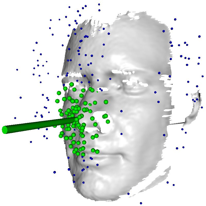
sum of the differential entropies computed at the children
PL and PR :

        IG = H(P) − (wL H(PL ) + wR H(PR )),                 (2)

where Pi∈{L,R} is the set of patches reaching node i and
wi is the ratio between the number of patches in i and in its
parent node, i.e., wi = |P i|
                         |P| .
    We model the vectors θ at each node as realizations of a
random variable with a multivariate Gaussian distribution,
i.e., p(θ) = N (θ; θ, Σ). Therefore, Eq. (2) can be rewritten
                                                                          Figure 4. Example test image: the green spheres are the ones se-
as:
                                                                          lected after the filtering of the outliers (blue spheres) by mean shift.
                               X                                          The large green cylinder stretches from the final estimate of the
         IG = log |Σ(P)| −          wi log |Σi (Pi )|.    (3)
                                                                          nose center in the estimated face direction.
                              i∈{L,R}

Maximizing Eq. (3) favors tests which minimize the deter-
minant of the covariance matrix Σ, thus decreasing the un-
certainty in the votes for the output parameters cast by each             PCA model constructed from aligned range scans of many
patch cluster.                                                            different people [22]. The initialization for the mean-shift
   Weassume the    covariance matrix to be block-diagonal               step is the mean of all votes returned by the forest, which
         Σv 0                                                             we assume to be close to the true nose location, where most
Σ=                    , i.e., we allow covariance only among              of the votes usually cluster. In our experiments, removing
          0 Σa
offset vectors (Σ ) and among head rotation angles (Σa ),
                   v                                                      outliers has shown to be crucial in test images where the
but not between them. Eq. (3) thus becomes:                               head undergoes large rotations and/or is partially occluded
                                                                          by glasses or facial hair. We finally sum all the remaining
                                                                          random variables θ, producing a Gaussian whose mean is
                                  X
 IG = log (|Σv | + |Σa |) −             wi log (|Σvi | + |Σai |).
                               i∈{L,R}
                                                                          the ultimate estimate of our output parameters and whose
                                                          (4)             covariance represents a measure of the estimate’s uncer-
   A leaf l is created when the maximum depth is reached                  tainty. An example test frame is shown in Fig. 4, where the
or a minimum number of patches are left. Each leaf stores                 small blue spheres are all votes cast by the forest, and the
the mean of all angles and offset vectors which reached it,               green, larger ones represent the votes selected after mean-
together with their covariance, i.e., a multivariate Gaussian             shift. The final estimate of the nose position and head di-
distribution.                                                             rection is represented by the green cylinder.

3.3. Testing
                                                                          3.4. Training Data Generation
    Given a new, unseen range image of a head, patches (of
the same size as the ones used for training) are densely sam-                 Random forests can be built from large training datasets
pled and passed through all trees in the forest. At each node             in reasonable time and are very powerful in learning the
of a tree, the stored binary test evaluates a patch, sending              most distinctive features for the problem at hand. We there-
it either to the right or left child, all the way down un-                fore generated a large database of 50K, 640x480 range im-
til a leaf. Arrived at a leaf l, a patch gives an estimate                ages of faces by rendering a 3D morphable model [22] in
for the pose parameters in terms of the stored distribution               many randomly generated poses. The rotations span ±95 ◦
p(θ|l) = N (θ; θ, Σ).                                                     for yaw, ±50 ◦ for pitch, and ±20 ◦ for roll. Moreover, we
    Because leaves with a high variance are not very infor-               randomly translated the 3D model along the z axis within a
mative and add mainly noise to the estimate, we discard                   50 cm range. We further perturbed the first 30 PCA modes
all Gaussians with a total variance greater than an empiric               of the shape model by ±2 of the standard deviation of each
threshold maxv . We also first locate the nose position to                mode, thus introducing random variations also in the iden-
remove outliers before estimating all other parameters. We                tity of the faces. We stored the 3D coordinates of each vis-
thus perform 10 mean-shift [7] iterations using a spherical               ible point on the face surface for each pixel in each image,
kernel and keep only the random variables whose means fall                together with the ground truth 3D coordinates of the nose
within the mean-shift kernel. The kernel radius is defined as             tip and the three rotation angles. Figure 5 shows a few of
a fraction of the size of the smallest sphere enclosing the av-           the training faces, with the red bar pointing out from the
erage human face, which we consider to be the mean of the                 nose indicating the head direction.

                                                                    620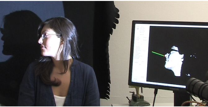
rors. We picked the values maxv = 400 and ratio = 5 as
                                                                            they showed the best compromise for the errors in both the
                                                                            nose localization and angle estimation task. Additionally,
                                                                            the number of trees to be used and a stride in the sampling
                                                                            of the patches for testing can be adapted to find the desired
                                                                            balance between accuracy and speed of the estimation pro-
                                                                            cess. This is a very important feature of our system since
                                                                            it allows to adapt the algorithm to the computational con-
                                                                            straints imposed by the application.
                                                                                In the following experiments, we always trained each
                                                                            tree sampling 25 patches from each of 3000 synthetically
                                                                            generated images, while the full ETH database was used
Figure 5. Sample images from our synthetically generated train-
ing set. The heads show large 3D rotations and variations in the
                                                                            for testing.
distance from the camera and also in identity. The red cylinder                 The plots in Fig. 6(a,d) show the time in ms needed to
attached to the nose represents the ground truth orientation of the         process one frame (once loaded into memory) using our
face.                                                                       method, depending on the number of loaded trees and on
                                                                            the stride. It is important to note that the current implemen-
                                                                            tation is not optimized, and could greatly benefit from using
4. Experiments                                                              integral images, possibly reducing the computation time of
                                                                            a factor of 2. Fig. 6(a) plots the average runtime (computed
   In order to assess the performance of our algorithm on re-               over 500 frames) for a stride fixed to 20 as a function of
alistic data, we used the ETH Face Pose Range Image Data                    the number of trees, while in Fig. 6(d) 15 trees are loaded
Set [4]. The database contains over 10K range images of                     and the stride parameter changes. The red circular markers
20 people (3 females, 6 subjects recorded twice, with and                   represent the performance of the system when all available
without glasses) turning their head while captured at 28 fps                feature channels are employed (i.e., depth and geometric
by the range scanner of [27]. The images have a resolution                  normals), while the blue crosses refer to the setup where
of 640x480 pixels, and a face typically consists of around                  only the depth channel is used. We used a computer with an
150x200 pixels. The head pose range covers about ±90 ◦                      Intel Core i7 CPU @ 2.67GHz, without resorting to multi-
yaw and ±45 ◦ pitch rotations. The provided ground truth                    threading. It can be seen that, for a number of trees less or
for each image consists of the 3D nose tip coordinates and                  equal to 15 and a stride greater or equal to 20, both curves
the coordinates of a vector pointing in the face direction.                 are well below 40ms, i.e., we achieve framerates above 25
   Our system outputs real-valued estimates for the 3D nose                 frames per second. If not otherwise specified, the remaining
location and the three head rotation angles. However, the                   results and images have been produced using these values
above database does not contain roll rotations, which are                   for the number of trees and the stride.
not encoded in the directional vector provided as ground                        The additional computations needed to extract the nor-
truth. Therefore, we evaluated our performance with regard                  mals (a 4-neighborhood is used - all done on the CPU)
to orientation by computing the head direction vector from                  pay off in terms of estimation accuracy, as visualized in the
the estimated yaw and pitch angles and report the angular                   Figs. 6(b,c,e,f). The plot in Fig. 6(b) shows the percentage
error with the vector provided as ground truth. For the nose                of correctly estimated images as a function of the success
localization, the Euclidian distance is used as error measure.              threshold set for the angular error, while in Fig. 6(e) the
   Our method is controlled by a few parameters. In the                     thresholds are defined on the nose localization error. As can
present setup, some parameters have been fixed intuitively,                 be seen in all plots, using all the available feature channels
like the size of the patches (120x80 pixels), the maximum                   performs consistently better than taking only the depth in-
size of the sub-patches defining the areas F1 and F2 in the                 formation. More in detail, for a conservative threshold of
tests (fixed to 40 pixels), and the number of mean-shift it-                10 ◦ on the angular error, our method succeeded in 90.4%
erations used to remove outliers from the set of random                     of the cases, 95.4% for 15 ◦ , and 95.9% for 20 ◦ . With the
variables obtained from the regression forest, set to 10.                   same thresholding and on the same dataset, [4] reports per-
Additional parameters are the maximum accepted variance                     centages of 80.8%, 97.8%, and 98.4%, i.e., we have im-
maxv of the Gaussians output of the leaves and the ratio                    proved the accuracy of about 10% for the most conservative
defining the radius of the mean-shift spherical kernel. In                  threshold, which is also the most relevant one. The perfor-
order to find the best combination of these last two param-                 mance for nose localization is shown in Fig. 6(e) where the
eters, we used a small part of the ETH database (1000 im-                   success rate for thresholds between 10 and 35 mm is plotted,
ages) and ran a coarse grid search for the best average er-                 e.g., setting a 20 mm threshold leads to 93.2% accuracy.

                                                                      621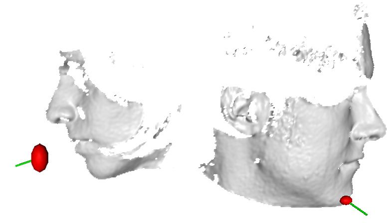
50 100 25
45
95
40
Average nose error (mm)
35
90 20
Runtime (ms)
30
Accuracy %
25 85
20
80 15
15
10
75
5 depth + normals
depth + normals
depth only depth only
0 70 10
5 10 15 20 25 10 12 14 16 18 20 5 10 15 20 25
# Trees (stride 20) Angle error (degrees) − 15 trees − stride 20 # Trees (stride 20)
(a) (b) (c)
100 100 25
depth + normals
90 depth only
90
80
Average nose error (mm)
70 20
80
Runtime (ms)
60
Accuracy %
50 70
40
60 15
30
20
50
10 depth + normals
depth only
0 40 10
10 15 20 25 30 10 15 20 25 30 35 10 15 20 25 30
Stride (15 trees) Nose error (mm) − 15 trees − stride 20 Stride (15 trees)
(d) (e) (f)
Figure 6. All plots are labeled in blue and crosses when only the depth channel is used by the system, and in red and circles when all four
channels are used (depth plus X,Y, and Z components of the normals). a) Regression time as a function of the number of trees in the forest
when the stride is fixed to 20 pixels, the reported values are averaged over 500 images. b) Accuracy of the system in terms of percentage
of correctly estimated poses as a function of the angle error threshold. c) Average nose error in mm, as a function of the number of trees
(with stride=20). d) Runtime of the system for a forest of 15 trees as a function of the stride parameter. e) Accuracy plotted against nose
error thresholds in mm. f) Nose localization error for a forest of 15 trees and varying stride. In the current, unoptimized settings, the
system achieves real-time performance for forests with ≤ 15 trees and a stride ≥ 20. The additional information coming from the normals
consistently boosts the performance.
Nose error Yaw error Pitch error Direction estimation accuracy
Our approach 13.4/21.1 mm 5.7/15.2 ◦ 5.1/4.9 ◦ 90.4%
Breitenstein et al. 9.0/14.0 mm 6.1/10.3 ◦ 4.2/3.9 ◦ 80.8%
Table 1. Comparison of our results with [4]. The first three columns show mean and standard deviation for the Euclidean error in the nose
tip localization task (mm) and for the yaw and pitch estimation (degrees). The values in the last column are the percentages of correctly
estimated images for a threshold on the angular error (to the ground truth provided with the ETH database) of 10 degrees.
In 6.5% of the range images in the ETH database, our ported by [4] are computed only on estimates with a high
system did not return an estimate, i.e., no votes were left nose detection confidence (positive rate of 80% and a false
under the mean-shift kernel; these images were discarded positive rate of 3%), but the percentage of retained images
before computing the following average errors. Figs. 6(c,f) is not provided. The last column of Table 1 is instead a fair
show the average error in the nose localization task, plot- comparison of the two systems because both values were
ted as a function of the number of trees when the stride is computed on the full ETH database, showing the percent-
fixed to 20 (6(c)) and as a function of the stride when 15 age of correctly classified images assuming a 10 ◦ threshold
trees are used (6(f)). Again, using the normals in addition to on the angular error.
the depth channel (red curve) shows considerably superior
performance. The mean and standard deviation of the pose Fig. 7 shows the success rate when the angle error thresh-
estimation error are reported in Table 1 and compared to the old is set to 15 ◦ , and the nose error to 20 mm. In this case,
errors reported in [4]. However, the first three columns of we loaded 15 trees as before, but set the stride to 10. The
Table 1 are not directly comparable, because the errors re- test dataset was divided based on the heads’ angles of rota-
tions for pitch and yaw, in areas of 15 ◦ × 15 ◦ . Only areas
622Figure 9. Example failure images from the ETH database. The
large ellipse denotes that the regression predicted a high variance
Figure 7. Normalized success rates of the estimation. The database for the estimate of the nose location.
was discretized in 15 ◦ × 15 ◦ areas and the accuracy compute for
each range of angles separately. The color encodes the number of
images falling in each region, as explained by the bar on the side.
direction. Our system is robust to large rotations and partial
facial occlusions (note the girl at the bottom right, with most
of the face covered by hair, which is not reconstructed by
with more than 10 images were considered and are filled in the scanner). Two example failures are rendered in Fig. 9.
the image; the color-coding represents the amount of data We ran our real-time system on a Intel Core 2 Duo com-
contained in the angle range of each area, as described by puter @ 2GHz, equipped with 2GB of RAM, which was
the color bar on the right. It can be noted how the results are simultaneously used to acquire the range data as explained
close to 100% for the central region of the map, where most in [27]. Fig. 10 shows some example frames, with our
of the images in the ETH database fall. The performance method successfully estimating the head pose even when
usually decreases in the corner regions, where the rotations the nose is badly occluded and thus most of the other ap-
are very large, and the number of images low. In general, proaches based on 3D data would fail. Facial expressions
our results are comparable to a similar plot presented in [4]. also do not seem to cause problems to the regression in most
of the cases, even though the synthetic training dataset con-
tains only neutral faces.
5. Conclusions
In this work, we have presented an approach for real-
time head pose estimation from depth data. In our exper-
iments, we have performed a thorough quantitative evalu-
ation on a publicly available database where our approach
achieves state-of-the-art performance. Because we do not
rely on specific hardware like a GPU, our approach is also
suitable for applications where hardware constraints limit
the computational resources. In particular, the introduction
of a stride for patch processing gives an easy-to-use parame-
ter to steer the trade-off between accuracy and computation
Figure 8. Correctly estimated poses from the ETH database. Large
cost for an optimal setting. Furthermore, our approach is ro-
rotations, glasses, and facial hair do not pose major problems in
most of the cases. The green cylinder represents the estimated
bust against severe occlusions, because we do not localize a
head rotation, while the red ellipse is centered on the estimated 3D few, specific facial features but estimate the pose parameters
nose position and scaled according to the covariance provided by from all surface patches within a regression framework.
the forest (scaled by a factor of 10 to ease the visualization).
6. Acknowledgements
Fig. 8 shows some successfully processed frames from The authors acknowledge financial support from the
the ETH database. The red ellipse represents the estimated SNF project Vision-supported Speech-based Human Ma-
nose location and it is scaled according to the covariance chine Interaction (200021-130224) and the EU project
output of the regression forest. The green cylinder is cen- RADHAR (FP7-ICT-248873). We also thank Thibaut
tered on the nose tip and stretches along the estimated head Weise for providing the 3D scanner and useful code.
623Figure 10. Example frames from our real-time head pose estimation system, showing how the regression works even in the presence of
facial expressions and partial occlusions.
References [15] S. Malassiotis and M. G. Strintzis. Robust real-time 3d
head pose estimation from range data. Pattern Recognition,
[1] V. N. Balasubramanian, J. Ye, and S. Panchanathan. Biased 38:1153 – 1165, 2005.
manifold embedding: A framework for person-independent [16] Y. Matsumoto and A. Zelinsky. An algorithm for real-time
head pose estimation. In CVPR, 2007. stereo vision implementation of head pose and gaze direction
[2] L. Breiman. Random forests. Machine Learning, 45(1):5– measurement. In Aut. Face and Gestures Rec., 2000.
32, 2001. [17] A. Mian, M. Bennamoun, and R. Owens. Automatic 3d face
[3] L. Breiman, J. Friedman, R. Olshen, and C. Stone. Classifi- detection, normalization and recognition. In 3DPVT, 2006.
cation and Regression Trees. Wadsworth and Brooks, Mon- [18] L.-P. Morency, P. Sundberg, and T. Darrell. Pose estimation
terey, CA, 1984. using 3d view-based eigenspaces. In Aut. Face and Gestures
[4] M. D. Breitenstein, D. Kuettel, T. Weise, L. Van Gool, and Rec., 2003.
H. Pfister. Real-time face pose estimation from single range [19] E. Murphy-Chutorian and M. Trivedi. Head pose estimation
images. In CVPR, 2008. in computer vision: A survey. TPAMI, 31(4):607–626, 2009.
[20] R. Okada. Discriminative generalized hough transform for
[5] Q. Cai, D. Gallup, C. Zhang, and Z. Zhang. 3d deformable
object dectection. In ICCV, 2009.
face tracking with a commodity depth camera. In ECCV,
2010. [21] M. Osadchy, M. L. Miller, and Y. LeCun. Synergistic face
detection and pose estimation with energy-based models. In
[6] L. Chen, L. Zhang, Y. Hu, M. Li, and H. Zhang. Head pose NIPS, 2005.
estimation using fisher manifold learning. In Workshop on
[22] P. Paysan, R. Knothe, B. Amberg, S. Romdhani, and T. Vet-
Analysis and Modeling of Faces and Gestures, 2003.
ter. A 3d face model for pose and illumination invariant face
[7] Y. Cheng. Mean shift, mode seeking, and clustering. TPAMI, recognition. In Advanced Video and Signal based Surveil-
17:790–799, 1995. lance, 2009.
[8] T. F. Cootes, G. J. Edwards, and C. J. Taylor. Active appear- [23] K. Ramnath, S. Koterba, J. Xiao, C. Hu, I. Matthews,
ance models. TPAMI, 23:681–685, 2001. S. Baker, J. Cohn, and T. Kanade. Multi-view aam fitting
[9] T. F. Cootes, G. V. Wheeler, K. N. Walker, and C. J. Tay- and construction. IJCV, 76:183–204, 2008.
lor. View-based active appearance models. Image and Vision [24] E. Seemann, K. Nickel, and R. Stiefelhagen. Head pose es-
Computing, 20(9-10):657–664, 2002. timation using stereo vision for human-robot interaction. In
[10] A. Criminisi, J. Shotton, D. Robertson, and E. Konukoglu. Aut. Face and Gestures Rec., 2004.
Regression forests for efficient anatomy detection and local- [25] M. Storer, M. Urschler, and H. Bischof. 3d-mam: 3d mor-
ization in ct studies. In Medical Computer Vision Workshop, phable appearance model for efficient fine head pose estima-
2010. tion from still images. In Workshop on Subspace Methods,
2009.
[11] J. Gall, A. Yao, N. Razavi, L. Van Gool, and V. Lempit-
[26] T. Vatahska, M. Bennewitz, and S. Behnke. Feature-based
sky. Hough forests for object detection, tracking, and action
head pose estimation from images. In Humanoids, 2007.
recognition. TPAMI, 2011.
[27] T. Weise, B. Leibe, and L. Van Gool. Fast 3d scanning with
[12] C. Huang, X. Ding, and C. Fang. Head pose estimation based automatic motion compensation. In CVPR, 2007.
on random forests for multiclass classification. In ICPR, [28] J. Whitehill and J. R. Movellan. A discriminative approach
2010. to frame-by-frame head pose tracking. In Aut. Face and Ges-
[13] M. Jones and P. Viola. Fast multi-view face detection. Tech- tures Rec., 2008.
nical Report TR2003-096, Mitsubishi Electric Research Lab- [29] R. Yang and Z. Zhang. Model-based head pose tracking with
oratories, 2003. stereovision. Aut. Face and Gestures Rec., 2002.
[14] V. Lepetit and P. Fua. Keypoint recognition using random- [30] J. Yao and W. K. Cham. Efficient model-based linear head
ized trees. TPAMI, 28:1465–1479, 2006. motion recovery from movies. In CVPR, 2004.
624You can also read