Recoding latent sentence representations

MS C A RTIFICIAL I NTELLIGENCE
 M ASTER T HESIS
arXiv:2101.00674v1 [cs.CL] 3 Jan 2021

 Recoding latent sentence
 representations
 Dynamic gradient-based activation modification in RNNs

 by

 D ENNIS U LMER
 11733187

 August 9, 2019
 36 ECTS
 January 2019 - August 2019

 Supervisors: Assessor:
 D IEUWKE H UPKES Dr. W ILLEM Z UIDEMA
 Dr. E LIA B RUNI

 I NSTITUTE FOR L OGIC , L ANGUAGE AND C OMPUTATION
 U NIVERSITY OF A MSTERDAM

Abstract

In Recurrent Neural Networks (RNNs), encoding information in a suboptimal or
erroneous way can impact the quality of representations based on later elements
in the sequence and subsequently lead to wrong predictions and a worse model
performance. In humans, challenging cases like garden path sentences (an instance
of this being the infamous The horse raced past the barn fell) can lead their language
understanding astray. However, they are still able to correct their representation
accordingly and recover when new information is encountered. Inspired by this, I
propose an augmentation to standard RNNs in form of a gradient-based correction
mechanism: This way I hope to enable such models to dynamically adapt their
inner representation of a sentence, adding a way to correct deviations as soon as
they occur. This could therefore lead to more robust models using more flexible
representations, even during inference time.

The mechanism explored in this work is inspired by work of Giulianelli et al., 2018,
who demonstrated that activations in a LSTM can be corrected in order to recover
corrupted information (interventions). This is achieved by the usage of “Diagnostic
Classifiers” (DG) (Hupkes et al., 2018), linear models that can help to identify the
kind of information recurrent neural networks encode in their hidden representa-
tions and correct them using their gradients. In this thesis, I present a generalized
framework based on this idea to dynamically adapt hidden activations based on local
error signals (recoding) and implement it in form of a novel mechanism. I explore
signals which are either based directly on the task’s objective or on the model’s
confidence, leveraging recent techniques from Bayesian Deep Learning (Gal and
Ghahramani, 2016b; Gal and Ghahramani, 2016a; Pearce et al., 2018).

Crucially, these updates take place on an activation rather than a parameter level
and are performed during training and testing alike. I conduct different experiments
in the context of language modeling, where the impact of using such a mechanism is
examined in detail.

To this end, I look at modifications based on different kinds of time-dependent error
signals and how they influence the model performance. Furthermore, this work
contains a study of the model’s confidence in its predictions during training and for
challenging test samples and the effect of the manipulation thereof. Lastly, I also
study the difference in behavior of these novel models compared to a standard LSTM
baseline and investigate error cases in detail to identify points of future research. I
show that while the proposed approach comes with promising theoretical guarantees
and an appealing intuition, it is only able to produce minor improvements over the
baseline due to challenges in its practical application and the efficacy of the tested
model variants.

 4

Acknowledgements

 春风化雨 - Spring wind and rain

 Chinese idiom about the merits of higher education

 Amsterdam, August 9, 2019

Nobody in this world succeeds alone. Giraffe calves are able to walk around on their
own within an hour after their birth, while the whole process takes human babies
around a year. And even then they require intense parental care throughout infancy,
and, in modern society, often depend on others way into their adulthood.
In the end, the essence of our own personality is distilled from the sum of all of our
experiences, which includes all the interactions we have with others. This forms a
giant, chaotic and beautiful network of beings, constantly in flux. I therefore owe
myself to the ones around me, a selection of which I want to thank at this point.

First and foremost, I want to thank my supervisors Dieuwke and Elia. Not only have
they fulfilled their duties as such with excellence by providing guidance and constant
feedback, they were also always available when I had questions or expressed doubts.
They furthermore gave me the opportunity to participate in research projects and
encouraged me to attend conferences and publish findings, essentially supporting
my first steps into academia. I also want to thank Willem Zuidema for taking his
time in assessing my thesis and taking part in my defense.

Secondly, I would like express my eternal gratitude to my family for all the ways
that they have supported my throughout my entire life in a myriad of ways. My
grandma Ingrid, my father Siegfried and my sister Anna; thank you for believing
in me and supporting me and providing me with the opportunity to develop follow
my interests. I want to especially thank my mother Michaela for constantly trying to
enkindle my curiosity when growing up, always nudging me into the right direction

during my teenage years and offering guidance to this very day.

Next, I would like to thank all my friends who contributed to this work and the past
two years of my life in a manifold of ways: Thank you Anna, Christina, Raj and
Santhosh for all those beautiful memories that I will be fondly remembering for the
rest of my life as soon as my mind reminisces about my time here in Amsterdam.
Futhermore, thank you Caro for holding me accountable and being a pain in the neck
of my inertia, and living through the highs and lows of the last two years. Thank
you Putri for getting me addicted to coffee, something I had resisted to my whole
life up until this point and for providing company in a costantly emptying Science
Park. Also, thank you Mirthe for applying mathematical rigour to my derivations
and to Atilla for being a super-human proof-reader.

I could extend this list forever but I have to leave some pages for my actual thesis,
therefore let me state the following: Although you might have stayed unmentioned
throughout this text, your contribution has not stayed unnoticed. And for the case
that I have not made my appreciation to you explicit: Thank you. I am grateful
beyond measure to be surrounded by some many great people that have supported
me in times of doubt and that I know that I can always turn to and the many more
that have enriched my life in smaller ways.

 7

List of Abbreviations

BAE Bayesian Anchored Ensembling. 18, 45, 51–54, 56–58, 62, 63, 65, 88

BPTT Backpropagation Through Time. 29

DC Diagnostic Classifier. 22, 38

DNN Deep Neural Network. 17, 25

ELBO Evidence Lower Bound. 32, 72, 73

HMM Hidden Markov Model. 17

LSTM Long-Short Term Memory. 21, 22, 29, 30, 37–39, 44, 48, 49, 56, 61, 69

MAP Maximum a posteriori. 12, 23, 32, 36, 37, 74

MCD Monte Carlo Dropout. 12, 33, 51–53, 56–58, 62, 63, 65, 66, 88

MLE Maximum Likelihood Estimate. 31

MLP Multi-Layer Perceptron. 17, 28, 34, 43, 45, 56, 66

MSE Minimum Squared Error (loss). 26

NN Neural Network. 37

PTB Penn Treebank. 48, 51, 53, 54, 61, 88

ReLU Rectified Linear Unit. 26, 56

RNN Recurrent Neural Network. 10, 12, 17–19, 21, 28–30, 34, 35, 39, 40, 44, 45,
 50, 66

 9

Contents

1 Introduction 16
 1.1 Research Questions . . . . . . . . . . . . . . . . . . . . . . . . . . . . 18
 1.2 Contributions . . . . . . . . . . . . . . . . . . . . . . . . . . . . . . . 19
 1.3 Thesis structure . . . . . . . . . . . . . . . . . . . . . . . . . . . . . . 20

2 Related Work 21
 2.1 Recurrent Neural Networks & Language . . . . . . . . . . . . . . . . 21
 2.2 Model Uncertainty . . . . . . . . . . . . . . . . . . . . . . . . . . . . 22
 2.3 Dynamic Models & Representations . . . . . . . . . . . . . . . . . . . 23

3 Background 25
 3.1 Deep Learning . . . . . . . . . . . . . . . . . . . . . . . . . . . . . . 25
 3.2 Recurrent Neural Language Models . . . . . . . . . . . . . . . . . . . 28
 3.2.1 Recurrent Neural Networks . . . . . . . . . . . . . . . . . . . 28
 3.2.2 Language Modeling with RNNs . . . . . . . . . . . . . . . . . 30
 3.3 Bayesian Deep Learning . . . . . . . . . . . . . . . . . . . . . . . . . 31
 3.3.1 Variational inference . . . . . . . . . . . . . . . . . . . . . . . 31
 3.3.2 Estimating model confidence with Dropout . . . . . . . . . . 33
 3.3.3 Estimating model confidence with ensembles . . . . . . . . . 35
 3.4 Recap . . . . . . . . . . . . . . . . . . . . . . . . . . . . . . . . . . . 37

4 Recoding Framework 38
 4.1 Interventions . . . . . . . . . . . . . . . . . . . . . . . . . . . . . . . 38
 4.2 Recoding Mechanism . . . . . . . . . . . . . . . . . . . . . . . . . . . 39
 4.3 Error Signals . . . . . . . . . . . . . . . . . . . . . . . . . . . . . . . 41
 4.3.1 Weak Supervision . . . . . . . . . . . . . . . . . . . . . . . . . 41
 4.3.2 Surprisal . . . . . . . . . . . . . . . . . . . . . . . . . . . . . . 41
 4.3.3 MC Dropout . . . . . . . . . . . . . . . . . . . . . . . . . . . . 43
 4.3.4 Bayesian Anchored Ensembling . . . . . . . . . . . . . . . . . 45
 4.4 Step Size . . . . . . . . . . . . . . . . . . . . . . . . . . . . . . . . . 46
 4.5 Recap . . . . . . . . . . . . . . . . . . . . . . . . . . . . . . . . . . . 46

5 Experiments 48
 5.1 Dataset . . . . . . . . . . . . . . . . . . . . . . . . . . . . . . . . . . 48
 5.2 Training . . . . . . . . . . . . . . . . . . . . . . . . . . . . . . . . . . 48

 10

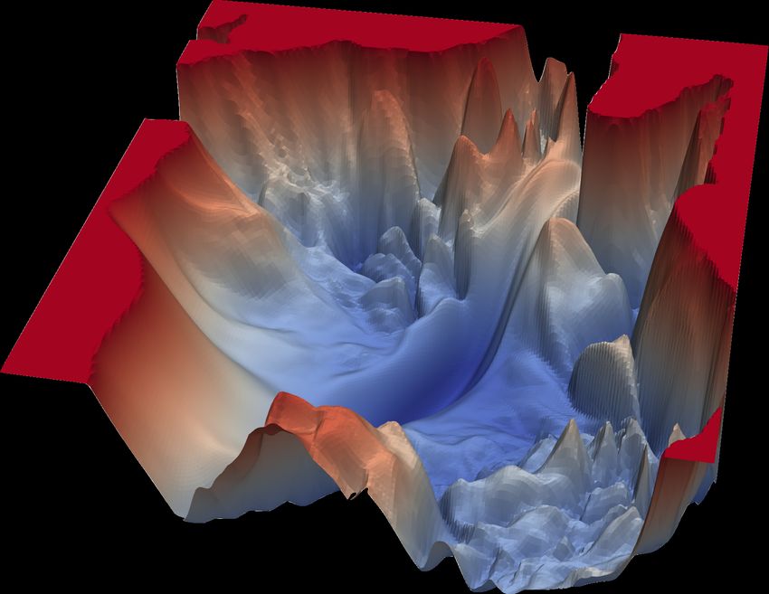
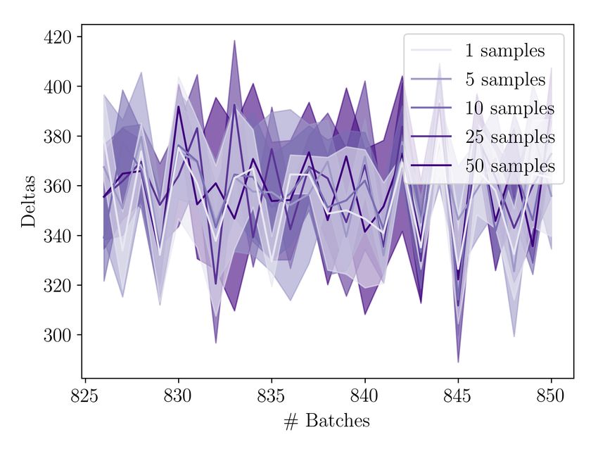
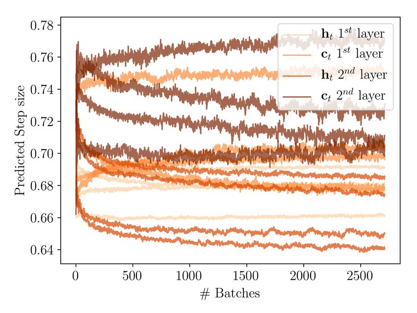
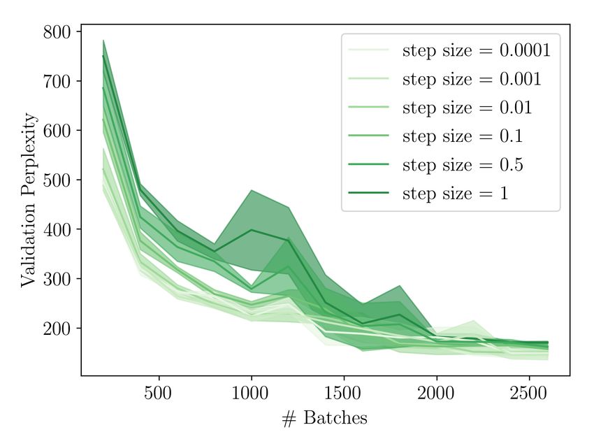
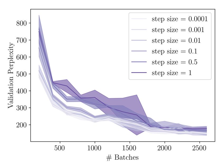
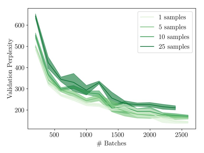
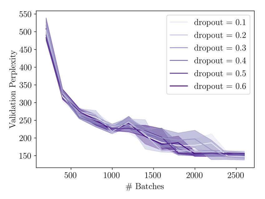
5.3 Evaluation . . . . . . . . . . . . . . . . . . . . . . . . . . . . . . . . . 50
 5.3.1 Recoding Step Size . . . . . . . . . . . . . . . . . . . . . . . . 50
 5.3.2 Number of samples . . . . . . . . . . . . . . . . . . . . . . . . 53
 5.3.3 MC Dropout rate . . . . . . . . . . . . . . . . . . . . . . . . . 55
 5.3.4 Dynamic Step Size . . . . . . . . . . . . . . . . . . . . . . . . 56
 5.3.5 Ablation . . . . . . . . . . . . . . . . . . . . . . . . . . . . . . 57

6 Qualitative Analysis 59
 6.1 Recoding Behaviour . . . . . . . . . . . . . . . . . . . . . . . . . . . 59
 6.1.1 Cognitive Plausibility . . . . . . . . . . . . . . . . . . . . . . . 60
 6.1.2 Error signal reduction . . . . . . . . . . . . . . . . . . . . . . 61
 6.1.3 Effect of overconfident predictions . . . . . . . . . . . . . . . 62

7 Discussion 64
 7.1 Step Size . . . . . . . . . . . . . . . . . . . . . . . . . . . . . . . . . 64
 7.2 Role of Error Signal . . . . . . . . . . . . . . . . . . . . . . . . . . . . 65
 7.3 Approximations & Simplifying Assumptions . . . . . . . . . . . . . . 65

8 Conclusion 67
 8.1 Future Work . . . . . . . . . . . . . . . . . . . . . . . . . . . . . . . . 67
 8.1.1 Recoding signals . . . . . . . . . . . . . . . . . . . . . . . . . 67
 8.1.2 Step size . . . . . . . . . . . . . . . . . . . . . . . . . . . . . . 68
 8.1.3 Efficiency . . . . . . . . . . . . . . . . . . . . . . . . . . . . . 68
 8.1.4 Training Procedure & Architecture . . . . . . . . . . . . . . . 69
 8.2 Outlook . . . . . . . . . . . . . . . . . . . . . . . . . . . . . . . . . . 69
 8.2.1 Innotivation over Scale . . . . . . . . . . . . . . . . . . . . . . 69
 8.2.2 Inspiration from Human Cognition . . . . . . . . . . . . . . . 70

Bibliography 72

A Lemmata, Theorems & Derivations 79
 A.1 Derivation of the Evidence lower bound . . . . . . . . . . . . . . . . 79
 A.2 Approximating Predictive Entropy . . . . . . . . . . . . . . . . . . . . 80
 A.3 Lipschitz Continuity . . . . . . . . . . . . . . . . . . . . . . . . . . . 82
 A.4 Theoretical guarantees of Recoding . . . . . . . . . . . . . . . . . . . 83
 A.5 Derivation of the Surprisal recoding gradient . . . . . . . . . . . . . . 86
 A.6 Derivations fo the Predictive Entropy recoding gradient . . . . . . . . 88

B Experimental Details & Supplementary Results 90
 B.1 Pseudocode . . . . . . . . . . . . . . . . . . . . . . . . . . . . . . . . 90
 B.2 Practical Considerations . . . . . . . . . . . . . . . . . . . . . . . . . 91
 B.3 Hyperparameter Search . . . . . . . . . . . . . . . . . . . . . . . . . 92
 B.4 Additional plots . . . . . . . . . . . . . . . . . . . . . . . . . . . . . . 93

 11

List of Tables

5.1 Test perplexities for different recoding step sizes . . . . . . . . . . . . . 52
5.2 Test perplexities for different numbers of samples . . . . . . . . . . . . 54

B.1 Training Hyperparameters . . . . . . . . . . . . . . . . . . . . . . . . . 92
B.2 Sample ranges for hyperparameter search . . . . . . . . . . . . . . . . 93

List of Figures

3.1 Visualized loss surfaces of two deep neural networks . . . . . . . . . . 27
3.2 Comparison of a common application of Dropout to RNNs with Gal and
 Ghahramani, 2016a . . . . . . . . . . . . . . . . . . . . . . . . . . . . . 34
3.3 Illustration of the randomized MAP sampling procedure . . . . . . . . 36

4.1 Illustration of the recoding framework . . . . . . . . . . . . . . . . . . 40
4.2 Illustration of different error signals. . . . . . . . . . . . . . . . . . . . 42

5.1 Training losses for different recoding step sizes . . . . . . . . . . . . . 51
5.2 Training losses for different numbers of samples . . . . . . . . . . . . . 53
5.3 Uncertainty estimates for different numbers of samples . . . . . . . . . 54
5.4 Results for using MCD recoding with different Dropout rates. . . . . . . 55
5.5 Overview over results with dynamic step size models. . . . . . . . . . . 57
5.6 Results for ablation experiments. . . . . . . . . . . . . . . . . . . . . . 58

6.1 Model surprisal scores on two garden path sentences . . . . . . . . . . 60
6.2 Error reduction through recoding on garden path sentences . . . . . . 62
6.3 The effect of uncertainty recoding on surprisal . . . . . . . . . . . . . . 63

B.1 Pseucode for Recoding with Surprisal . . . . . . . . . . . . . . . . . . . 90
B.2 Pseudocode for Recoding with MC Dropout . . . . . . . . . . . . . . . 91
B.3 Pseudocode for Recoding with Bayesian Anchored Ensembles . . . . . 94
B.4 Training loss for different dropout rates when using MCD recoding . . 95
B.5 Additional plots for dynamic step size models. . . . . . . . . . . . . . . 95

 12

B.6 Additional plots for error reduction through recoding on garden path
 sentences . . . . . . . . . . . . . . . . . . . . . . . . . . . . . . . . . . 96

 13

Note on Notation

In this short section I introduce some conventions about the mathematical notations
in this thesis. This effort aims to make the use of letters and symbols more consistent
and thereby avoid any confusion.

Statistics A random variable : Ω ↦→ is a function that maps a set of possible
outcomes Ω to measurable space . In this work, the measurable space always
corresponds to the set of real numbers R. Parallel to the conventions in the Machine
Learning research community, random variables are denoted using an uppercase
letter, while realizations of the random variable from are denoted with lowercase
letters = , ∈ . Furthermore, the probability of this realization is denoted
using a lowercase like in ( ), disregarding whether the underlying distribution is a
probability mass function (discrete case) or probability density function (continuous
case). In cases where a variable has multiple distributions (e.g. in the context of vari-
ational inference), another lowercase letter like ( ) is used. The same holds when
using conditional probabilites like ( | ). In case the lowercase realization is bolded,
the distribution is multivariate, e.g. (x). E[·], Var[·] denote the expected value and
variance of a random variable, while H[·] denotes the entropy of its corresponding
distribution. If no subscript is used for the expected value, we are evaluating the
expected value with respect to the same probability distribution; in other cases this
 ∫︀
is made explicit like in E ( ) [ ( )] = ( ) ( ) .

Linear Algebra Matrices are being denoted by using bold uppercase letters, e.g. A
or Γ, including the identity matrix, I. Vectors however are written using lowercase
bold letter like b. Scalars are simply written as lowercase letters like . Vector
norms are written using || . . . ||, using the subscript (∞) for the ∞ norm. With-
out subscripts, this notations corresponds to the euclidean norm or inner product
||x|| = (x x)1/2 = ⟨x, x⟩.

Parameters Throughout this work, sets of (learnable) model parameters are denoted
using bolded greek lowercase letters, where denotes the set of all model parameters

 14

and the set of all model weight matrices (without biases). In a slight abuse of
notation, these two symbols are also used in contexts where they symbolize a vector
of (all) parameters. In case a function is parameterized by a set of parameters, this
is indicated by adding them as a subscript, e.g. (·).

Indices, Sets & Sequences When using indexed elements, the lowercase letter is
used for some element of an indexed sequence while the uppercase letter denotes
the highest index, like 1 . . . , , . . . . The only exception to this is the index ,
where is used to write the total number of elements indexed by . The index 
is exclusively used to denote time. Sets of elements are written using a shorthand
{ } 1 = { 1 , . . . , , . . . , }. In case the elements are ordered, a sequence is
written similarly using ⟨ ⟩ 1 = ⟨ 1 , . . . , , . . . , ⟩. Both sets and sequences are
written using caligraphic letters like or . In case of sets or sequences are used for
probalities or function arguments, the brackets are omitted completely for readability,
as in ( 1 ) = ( 1 , . . . , , . . . , )

Superscripts ·* is used to denote the best realization of some variable or parameter.
·′ is used to signifies some new, modified or updated version. ^· denotes an estimate,
while ˜· is used for approximations or preliminary values. And index in parenthesis
like ·( ) indicates the membership to some group or set.

Functions Here I simply list a short description of the most commonly used functions
in this work:

 • exp(·): Exponential function with base 

 • log(·), log2 (·): Natural and base 2 logarithm

 • (·|·, ·): Uni- or multivariate normal distribution

 • Bernoulli(·): Bernoulli distribution

 • 1(·): Indicator function
 • KL[·||·]: Kullback-Leibler divergence

 • ℒ(·): Some loss function used for neural network training

 • ELBO[·]: Evidence lower bound of a probability distribution

 15

Introduction 1
 “Language is perhaps our greatest accomplishment as a
 species. Once a people have established a language, they
 have a series of agreements on how to label, characterize,
 and categorize the world around them [...]. These
 agreements then serve as the foundation for all other
 agreements in society. Rosseau’s social contract is not the first
 contractual foundation of human society [...]. Language is."

 Don’t sleep, there are snakes - David Everett

Language forms the basis of most human communication. It enables abstract reason-
ing, the expression of thought and the transfer of knowledge from one individual
to another. It also seems to be a constant across all human languages that their
expressivity is infinite, i.e. that there is an infinite amount of possible sentences in
every human language (Hauser et al., 2002).1 Furthermore, natural language is
often also ambiguous and messy (Sapir, 1921) and relies on the recipient to derive
the right meaning from context (Chomsky, 1956; Grice et al., 1975), a fact that
distinguishes it from unambiguous artificial or context-free languages like predicate
logic or some programming languages (Ginsburg, 1966). It might therefore seem
surprising that humans - given the constraints in time and memory they face when
processing language - are able to do successfully. How they do so is still far from
being fully understood, which is why it might be helpful to study instances which
challenge human language processing.

As an example, take the following sentence: “The old man the boat” is an instance
of a phenomenon called garden-path sentences.2 These sentences are syntactically
challenging, because their beginning suggests a parse tree that turns out to be wrong
once they finish reading the sentence. In the end, it forces them to reconstruct the
sentence’s parse. In this particular instance, the sentence “The old man the boat”
seems to lack its main verb, until it is realized by the reader that “The old man”
is not a noun phrase consisting of determiner - adjective - noun but actually a verb
phrase based on “(to) man” as the main verb and “The old” as the sentence’s subject.

 1
 Although this also remains a controversial notion considering e.g. the Pirahã language, which seems
 to lack recursion (Everett et al., 2004). This is further discussed in Evans and Levinson, 2009, but
 not the intention of this work.
 2
 The name is derived from the idiom “(to) be led down the garden path”, as in being mislead or
 deceived.

 16

Humans are prone to these ambiguities (Christiansen and Chater, 2016; Tessler
et al., 2019), but display two interesting abilities when handling them:

 1. They process inputs based on some prior beliefs about the frequency and
 prevalence of a sentence’s syntactic patterns and semantics.

 2. They are able to adapt and correct their inner representation based on newly
 encountered, incrementally processed information.

Insights like these acquired in linguistics can enable progress in the field of compu-
tational linguistics, which tries to solve language-based problems with computers.
Since the surge of electronic computing in the 1940s, applying these powerful ma-
chines to difficult problems like automatic translation has been an active area of
research (Abney, 2007). While early works in natural language processing and other
subfields of artificial intelligence have focused on developing intricate symbolic
approaches (for an overview see e.g. Buchanan, 2005; Jurafsky, 2000), the need for
statistical solutions was realized over time. Early trailblazers of this trend can be
found in the work of Church, 1989 and DeRose, 1988, who apply so-called Hidden
Markov Models (HMMs) to the problem of Part-of-Speech tagging, i.e. assigning
categories to words in a sentence. Nowadays, the field remains deeply intertwined
with a new generation of statistical models: Artificial Neural Networks, also called
Deep Neural Networks (DNNs) or Multi-Layer Perceptrons (MLPs). These connec-
tonist models, trying to (very loosely) imitate the organization of neurons in the
human brain, are by no means a recent idea. With the first artificial neuron being
trained as early as the 1950s (Rosenblatt, 1958), effective algorithms to train several
layers of artificial cells connected in parallel were developed by Rumelhart et al.,
1988. However, after some fundamental criticisms (Minsky and Papert, 1969), this
line of research fell mostly dormant. Although another wave of related research
gained attraction in the 1980s and 1990s, it failed to meet expectations; only due
to the effort of some few researches combined with improved hardware and the
availability of bigger data sets, Deep Learning was able to produce several landmark
improvements (Bengio et al., 2015), which sent a ripple through adjacent fields,
including computational linguistics. Indicative for this is e.g. the work of Bengio
et al., 2003, developing a neural network-based Language Model, which was able to
outperform seasoned -gram approaches by a big margin and also introduced the
concept of word embeddings, i.e. the representation of words as learned, real-valued
vectors.

In recent years, Recurrent Neural Networks (RNNs) have developed into a popular
choice in Deep Learning to model sequential data, especially language. Although
fully attention-based models without recurrency (Vaswani et al., 2017; Radford
et al., 2018; Radford et al., 2019) have lately become a considerable alternative,

 17

RNN-based models still obtain state-of-the-art scores on tasks like Language Model-
ing (Gong et al., 2018), Sentiment Analysis (Howard and Ruder, 2018) and more.
However, they still lack the two aforementioned capabilities present in humans
when it comes to processing language: They do not take the uncertainty about
their predictions and representations into account and they are not able to correct
themselves based on new inputs.

The aim of this thesis is to augment a RNN architecture to address both of these
points: Firstly by developing a mechanism that corrects the model’s internal rep-
resentation of the input at every time step, similar to a human’s correction when
reading a garden path sentence. Secondly, this correction will be based on sev-
eral methods, some of which like Monte Carlo Dropout (MC Dropout) or Bayesian
Anchored Ensembling (BAE) were developed in a line of research called Bayesian
Deep Learning, which is concerned with incorporating bayesian statistics into Deep
Learning models. These methods help to quantify the degree of uncertainty in a
model when it is making a prediction and can be used in combination with the
correction mechanism to directly influence the amount of confidence the model has
about its internal representations.

1.1 Research Questions
Building on the ideas of uncertainty and self-correction, this thesis is concerned
with realizing them in a mathematical framework and followingly adapt the imple-
mentation of a RNN language model with a mechanism that performs the layed-out
adaptations of hidden representations. From this intention, the subsequent research
questions follow:

How to realize corrections? Gradient-based methods are a backbone of the success
of Deep Learning since the inception of the first artificial neurons in the 1950s
(Bengio et al., 2015) and its variants in their manifoldness still remain an important
tool in practice today.3 However, these methods are usually only applied to the
model parameters after processing a batch of data. Frequent local adaptions of
activations have - to the best of my knowledge - not been attempted or examined
in the literature, with the single exception of the paper this work draws inspiration
from (Giulianelli et al., 2018).

On what basis should corrections be performed? Another research question that
follows as a logical consequence of the previous one focuses on the issue of the
mechanism’s modality: The described idea requires to take the gradient of some
 3
 E.g. refer to Ruder, 2016 for an overview over the most frequently used gradient-based optimizers.

 1.1 Research Questions 18

“useful” quantity with respect to the network’s latent representations. This quantity
can e.g. spring from additional data as in Giulianelli et al., 2018, which results
in a partly supervised approach. This supervision requires additional information
about the task, which is not always available or suffers from all the problems that
come with manually labeling data on scale: The need for expertise (which might
not even produce handcrafted features that are helpful for models; deep neural
networks often find solutions that seem unexpected or even surprising to humans) as
well as a time- and resource-consuming process. This work thus examines different
unsupervised approaches based on a word’s perplexity and uncertainty measures
from the works of Gal and Ghahramani, 2016b; Gal and Ghahramani, 2016a; Pearce
et al., 2018.

What is the impact on training and inference? In the work of Giulianelli et al.,
2018, the idea has only been applied to a fully-trained model during test time. The
question still remains how using such an extended model would behave during
training as adapting activations in such a way will have a so far unstudied effect
on the learning dynamics of a model. Furthermore, it is the aim of this thesis to
also shed some light on the way that this procedure influences the model’s behavior
during inference compared to a baseline, which is going to be evaluated on a batch
and word-by-word scale.

1.2 Contributions
In this thesis I make the following contributions:

 • I formulate a novel and flexible framework for local gradient-based adaptions
 called recoding, including the proof of some theoretical guarantees.

 • I implement this new framework in the context of a recurrent neural language
 model.4

 • I examine potential sources of unsupervised “error signals” that trigger correc-
 tions of the model’s internal representations.

 • Finally, I provide an in-depth analysis of the effect of recoding on the model
 during training and inference as well as a validation of theoretical results and
 an error analysis.

 4
 The code is available online only under https://github.com/Kaleidophon/tenacious-toucan.

 1.2 Contributions 19

1.3 Thesis structure
The thesis is structured as follows: After this introduction, other relevant works
about the linguistic abilities of RNNs, Bayesian Deep Learning and more dynamic
deep networks are being summarized in chapter 2. Afterwards, I provide some
relevant background knowledge for the approaches outlined in this thesis in chapter
3, including a brief introduction to Deep Learning, Language Modeling with Re-
current Neural Networks and Bayesian Deep Learning. A formalization of the core
idea described above is given in chapter 4, where I develop several variants of its
implementations based on different error signals. These are subsequently evaluated
in an experimental setting in chapter 5, where the impact of the choice of hyper-
parameters concerning recoding and importance of different model components is
studied. A closer look at the behavior of the models on a word level is taken in
chapter 6. A full discussion of all experimental results is then given in chapter 7.
Lastly, all findings and implications of this work are summarized in chapter 8, giving
an outlook onto future research. Additional supplementary material concerning rele-
vant lemmata, extensive derivations and additional figures as well as more details
about the experimental setup are given in appendices A and B.

 1.3 Thesis structure 20

Related Work 2
 “The world (which some call the Library) is made up of an
 unknown, or perhaps unlimited, number of hexagonal
 galleries, each with a vast central ventilation shaft
 surrounded by a low railing. From any given hexagon, the
 higher and lower galleries can be seen stretching away
 interminably."

 The Library of Babel - Jorge Luis Borges

In this chapter I review some relevant works for this thesis regarding the linguistic
abilities of recurrent neural network models as well as the state-of-the-art approaches
for Language Modeling. A small discussion is dedicated to the role of some tech-
niques for “interpretable” artificial intelligence and the influences from the area of
Bayesian Deep Learning that are the foundation for the framework presented in
chapter 4. Lastly, I give an overview over a diverse set of ideas concerning more
dynamic models and representations.

2.1 Recurrent Neural Networks & Language
Recurrent Neural Networks (Rumelhart et al., 1988) have long been established as
a go-to architecture when modelling sequential data like handwriting (Fernandez
et al., 2009) or speech (Sak et al., 2014). One particularly popular variant of RNNs is
the Long-Short Term Memory Network (LSTM) (Hochreiter and Schmidhuber, 1997),
where the network learns to “forget” previous information and add new to a memory
cell, which is used in several gates to create the new hidden representation of the
input and functions as a sort of long-term memory. This has some special impli-
cations when applying recurrent networks to language-related tasks: It has been
shown that these networks are able to learn some degree of hierarchical structure
and exploit linguistic attributes (Liu et al., 2018), e.g. in the form of numerosity
(Linzen et al., 2016; Gulordava et al., 2018), nested recursion (Bernardy, 2018),
negative polarity items (Jumelet and Hupkes, 2018), or by learning entire artificial
context-free languages (Gers and Schmidhuber, 2001).

The most basic of language-based tasks lies in modeling the conditional probabilities
of words in a language, called Language Modeling. Current state-of-the-art mod-

 21

els follow two architectural paradigms: They either use a LSTM architecture, for
instance in the case of Gong et al., 2018 or use another popular attention-centric
approach which recently was able to produce impressive results. Attention, a mecha-
nism to complement a model in a way that is able to focus on specific inputs was
first introduced in the context of a recurrent encoder-decoder architecture (Bah-
danau et al., 2015). In the work of Vaswani et al., 2017, this was extended to a
fully (self-)attention-based architecture, which comprises no recurrent connections
whatsoever. Instead, the model uses several attention mechanisms between every
layer and makes additional smaller adjustments to the architecture to accommodate
this structural shift. This new model type was further extended in Dai et al., 2019
and most recently in Radford et al., 2019.

However, due to the sheer amount of parameters and general complexity of mod-
els, the way they arrive at their predictions is often not clear. In order to allow
the deployment of models in real-life scenarios with possible implications for the
security and well-being of others, it is thus of paramount importance to understand
the decision process and learned input representations of models (Brundage et al.,
2018). One such tool to provide these insights into the inner workings of a neural
network can be linear classifiers which are trained on the network’s activations to
predict some feature of interest (Hupkes et al., 2018; Dalvi et al., 2018; Conneau
et al., 2018), called Diagnostic Classifiers (DC). Giulianelli et al., 2018 use this
exact technique to extend the work of Gulordava et al., 2018 and show when in-
formation about the number of the sentence’s subject in LSTM activations is being
corrupted. They furthermore adjust the activations of the network based on the error
of the linear classifier and are thus able to avoid the loss of information in some cases.

2.2 Model Uncertainty
Standard Deep Learning approaches do not consider the uncertainty of model
predictions. This is especially critical in cases where deployed models are dele-
gated important and possibly life-affecting decisions, such as in self-driving cars or
medicine. Furthermore, incorporating the Bayesian perspective into Deep Learning
reduces the danger of making overly confident predictions (Blundell et al., 2015)
and allows for the consideration of prior beliefs to bias a model toward a desired
solution. Therefore, a line of research emerged in recent years trying to harmonize
established Deep Learning approaches with ideas from Bayesian inference. However,
ideas that try sample weights from learned distributions (Blundell et al., 2015)
are often unfeasible as they do not scale to the profound models and humongous
datasets utilized in practice.

 2.2 Model Uncertainty 22

An influential work managed to exploit a regularization technique called Dropout
(Srivastava et al., 2014), which deactives neurons randomly during training in order
to avoid overfitting the training data, to model the approximate variational distribu-
tion over the model weights (Gal and Ghahramani, 2016b), which in turn can be
used to estimate the predictive uncertainty of a model. These results have also been
extended to recurrent models (Gal and Ghahramani, 2016a) and successfully applied
in cases like time series prediction in a ride-sharing app (Zhu and Laptev, 2017).
Another promising approach to quantify uncertainty is exploiting model ensembles,
as shown in Lakshminarayanan et al., 2017, which forgoes the variational approach.
Technically, this approach cannot be considered Bayesian and was therefore extended
using a technique called Randomized Anchored MAP Sampling, where uncertainty
estimates can be procuded by employing an ensemble of Deep Neural Networks
regularized using the same anchor noise distribution (Pearce et al., 2018).

2.3 Dynamic Models & Representations
Lastly, there have also been some efforts to make models more adaptive to new data.
Traditionally, models parameters are adjusted during a designated training phase.
Afterwards, when a model is tested and then potentially deployed in a real-world
enviromment, these parameters stay fixed. This carries several disadvantages: If
the distribution of the data the model is confronted with differs from the training
distribution or changes over time, the model performance might drop. Therefore,
different lines of research are concerned with finding a solution that either enable
continuous learning (like observed in humans or animals) or more flexible represen-
tations.

Some works directly attack the problem of differing data distributions and the
transfer of knowledge across different domains (Kirkpatrick et al., 2017; Achille
et al., 2018). Further ideas about continuous learning have been explored under
the “Life-long learning” paradigm e.g. in Reinforcement Learning (Nagabandi et al.,
2019) or robotics (Koenig and Matarić, 2017). In Natural Language Processing, one
such idea consists of equipping a network with a self-managed external memory,
like in the works of Sukhbaatar et al., 2015 and Kaiser et al., 2017. This way allows
for a way to adjust hidden representations based on relevant information learned
during training. In contrast, the work of Krause et al., 2018 has helped models to
achieve state-of-the-art results in Language Modeling by making slight adjustments
to the models’ parameters when processing unseen data. It should be noted that
these approaches directly target model parameters, while this work is concerned
with adjusting model activations, which, to the best of my knowledge, has not been
attempted in the way that it is being presented here.

 2.3 Dynamic Models & Representations 23

The next chapter goes more into the technical details of related works.

 2.3 Dynamic Models & Representations 24

Background 3
 “As well as any human beings could, they knew what lay
 behind the cold, clicking, flashing face – miles and miles of
 face – of that giant computer. They had at least a vague
 notion of the general plan of relays and circuits that had long
 since grown past the point where any single human could
 possibly have a firm grasp of the whole. Multivac was
 self-adjusting and self-correcting. It had to be, for nothing
 human could adjust and correct it quickly enough or even
 adequately enough."

 The Last Question - Isaac Asimov

In this chapter, I supply the reader with some background knowledge relevant to the
content of this work, from the basic concepts of Deep Learning in section 3.1 and
their extension to language modeling in section 3.2. In section 3.3 I try to convey
the intuition of Bayesian Deep Learning, which helps to quantify the uncertainty in a
network’s prediction. I also outline approaches derived from it used in this thesis as
possible signals for activation corrections which approximate this very quantity.

3.1 Deep Learning
Deep Learning has achieved impressive results on several problems in recent years,
be it high-quality machine translation (Edunov et al., 2018), lip reading (Van Den
Oord et al., 2016), protein-folding (Evans et al., 2018) and beating human oppo-
nents in complex games like Go (Silver et al., 2016), just to name a few examples
among many. On a theoretical level, Deep Neural Networks (DNN) have been shown
to be able to approximate any continuous function under certain conditions (Hornik
et al., 1989; Csáji, 2001), which helps to explain their flexibility and success on
vastly different domains.

These DNNs consist of an arbitrary number of individual layers, each stacked upon
one another. The layers are feeding off increasingly complex features - internal,
learned representations of the model realized in real-valued vectors - that are the
output produced by the preceeding layer. A single layer in one of these networks can

 25

be described as an affine transformation of an input x with a non-linear activation
function applied to it

 x( +1) = (W( ) x( ) + b( ) ) (3.1)

where x( ) describes the input of the -th layer of the network and W( ) and b( )
are the weight and bias of the current layer, which are called learned parameters
of the model. Using a single weight vector w, this formulation corresponds to the
original Perceptron by Rosenblatt, 1958, a simple mathemathical model for a neuron
cell which weighs each incoming input with a single factor in order to obtain a
prediction. Using a weight matrix W therefore signifies using multiple artificial
neurons in parallel. The non-linear activation function (·) plays a pivotal role:
Stacking up linear transformation results in just another linear transformation in
the end, but by inserting non-linearities we can achieve the ability to approximate
arbitrary continuous functions like mentioned above. Popular choices of activation
functions include the sigmoid function, tangens hyperbolicus (tanh), the rectified
linear unit (ReLU) as well as the Softplus function, ReLU’s continuous counterpart:

 sigmoid( ) = (3.2)
 + 1

 2
 tanh( ) = −1 (3.3)
 1 + −2 

 relu( ) = max(0, ) (3.4)

 softplus( ) = log(1 + ) (3.5)

The network itself is typically improved by first computing and then trying to
minimize the value of an objective function or loss. This loss is usually defined as
the deviation of the model’s prediction from the ground truth, where minimizing
the loss implies improving the training objective (a good prediction). A popular
choice for this loss is the minimum squared error (MSE) loss, where we compute the
average squared distance between the models prediction ^ for a datapoint x and
the actual true prediction using the 2 -norm:

 1 ∑︁
 ℒMSE = || − ^ ||2 (3.6)
 =1

However in practice, many other loss functions are used depending on the task,
architecture and objective at hand. This loss can then be used by the Backpropagation

 3.1 Deep Learning 26

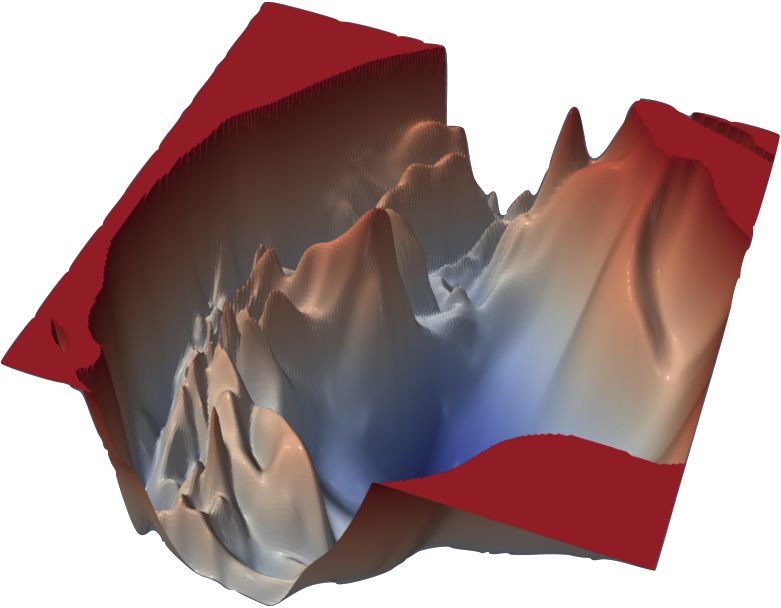
algorithm (Rumelhart et al., 1988), which recursively computes the gradient ∇ ℒMSE ,
a vector of all partial derivatives of the loss with respect to every single of the model’s
parameters . It is then used to move the same parameters into a direction which
minimizes the loss, commonly using the gradient descent update rule:

 ′ = − ∇ ℒMSE (3.7)

Figure 3.1.: Visualized loss surfaces of two deep neural networks. The “altitude” of the
 surfaces is determined by the value of the loss function the parameters of
 the models with the corresponding - and -values produce. This figure only
 depicts the projection of the loss surface into 3D space, as neural networks
 contain many more than just two parameters. Images taken from Li et al., 2018.
 Best viewed in color.

where is a positive learning rate with ∈ R+ . This effectively means that we
evaluate the quality of the network parameters at every step by looking at the
prediction they produced. The gradient points into the direction of steepest ascend.
Consequently, the antigradient (−∇ ℒMSE ) points us into the direction of the steep-
est descend. Updating the parameters into this direction means that we seek to
produce a set of new parameters ′ which theoretically decreases the value of the
loss function during the next step.

It is possible for convex loss functions to find their global minimum, i.e. the set of
parameters that produces a loss that is lower than all other possible losses, in a single
step (cp. Bishop, 2006 §3). However, as illustrated in figure 3.1, neural networks
are known to have highly non-convex loss functions - highly dimensional, rugged
loss surfaces with many local minima and an increasing number of saddle points as
the dimensionality of the parameter space (the number of parameters in the model)
increases (Dauphin et al., 2014). We therefore only take a step of length into the
direction of the antigradient. Using a suitable learning rate , this is guaranteed
to converge to a local minimum (Nesterov, 2018). Although this local mininum is
rarely the global minimum, the found solution often suffices to solve the task at
hand in a satisfactory manner.

 3.1 Deep Learning 27

3.2 Recurrent Neural Language Models
In this section I provide some insight into the motivation for and inner workings
of Recurrent Neural Networks (3.2.1), an extension to standard MLPs especially
suited for sequential data. Also, I outline their application to Language Modeling
(3.2.2), where we try to model the probability distribution that human language is
“generated” from and which will be the main objective of this thesis.

3.2.1 Recurrent Neural Networks
Recurrent Neural Networks (RNNs) are a special type of Deep Neural Networks which
comprises recurrent connections, meaning that they produce new representations
based on their prior representations. Due to this recurrent structure, they present
an inductive bias in their architecture which makes them especially suitable for
modeling sequences of data (Battaglia et al., 2018).

Formally, a sequence of input symbols like words is mapped to a sequence of
continuous input representations = ⟨x1 , . . . , x ⟩ with x ∈ R called embeddings,
real-valued vector representations for every possible symbol that is used as an input
to the model. When dealing with language, every word in the vocabulary of a corpus
is mapped to a word embedding. These representations are initialized randomly
and then tuned alongside the model’s parameters during training. Furthermore, a
recurrent function (·) parameterized by is used to compute hidden representations
h based on the current input representation x and the last hidden representation
h −1 with h ∈ R :

 h = (x , h −1 ) (3.8)

Considering that the hidden activations h depend on their predecessors thus allows
the RNN to capture information across multiple processing steps. This recurrent
function (·) can be realized in many different ways. In its simplest, most commonly
used form, it is stated as

 h = tanh(Wℎ x + bℎ + Wℎℎ h −1 + bℎℎ ) (3.9)

with = {Wℎ , Wℎℎ , bℎ , bℎℎ } as the learnable parameters. In a classification
setting, where we try to predict the most likely output category, we can produce a
categorical probability distribution over all possible classes in the following way: For
every hidden state h , an affine transformation is applied to create the distribution

 3.2 Recurrent Neural Language Models 28

over possible output symbols o (eq. 3.10) with o ∈ R| | , where denotes the
set of all symbols, or vocabulary. As this distribution usually does not meet the
requirements of a proper probability distribution, it is then typically normalized
using the softmax function, so that the total probability mass amounts to 1 (eq.
3.11)

 õ = Wℎ h + bℎ (3.10)

 exp(õ )
 o = ∑︀ (3.11)
 =1 exp(õ )

where Wℎ ∈ R| |× and bℎ ∈ R| | .

When training this kind of network, it is often observed that gradients shrink more
and more the longer the input sequence is, not allowing for any meaningful im-
provements of the parameters, which is called the vanishing gradient problem: When
calculating the gradients for the network’s parameters, a modification to the earlier
introduced backpropagation algorithm, backpropagation through time (BPTT) has
to be used, as the recurrency of the network conditions later outputs on earlier
processes. If we now evaluate the resulting product of partial derivatives, we often
find gradients to tend to zero when the network’s error is sufficiently small.1

The Long-Short Term Memory network (LSTM) by Hochreiter and Schmidhuber,
1997, which is the basis for the models used in this work, tries to avoid this problem
by augmenting the standard RNN recurrency by adding several gates:

 f = (Wℎ h −1 + W x + bℎ + b ) (3.12)

 i = (Wℎ h −1 + W x + bℎ + b ) (3.13)

 o = (Wℎ h −1 + W x + bℎ + b ) (3.14)

 c = f ∘ c −1 + i ∘ tanh(Wℎ h −1 + W x + bℎ + b ) (3.15)

 h = o · tanh(c ) (3.16)

 1
 Or in other words, lim ∇ ℒ = 0 holds for the gradient of the parameters and an input lag , i.e.
 →∞
 the number of time steps the error is being propagated back in time, if the spectral radius (or
 biggest absolute eigenvalue) of ∇ ℒ is smaller than one (Hochreiter et al., 2001).

 3.2 Recurrent Neural Language Models 29

which are called the forget gate f , input gate i and output gate o (not to be
confused with the output activations o ). A new type of activations, the cell state c ,
is also added. The activations of all gates consist of linear combinations of affine
transformations of the last hidden state h −1 and the current input x (eqs. (3.12)
to (3.14)).

However, each of them is assigned a different role within the cell’s architecture: The
input gate determines to which extent information is flowing into the cell state, the
forget gates modulates the amount of information inside the cell state that is being
erased and the output gate defines how much information flows from the cell state
to the new hidden state h (eq. 3.16). The role of the cell state c is to act as a form
of memory storage that is being updated based on the current input. Not only does
this enable the LSTM to model more long-term dependencies in its input sequence2 ,
the formulation of the cell state update in eq. 3.15 allows gradients to still “flow”
through the forget gate when computing the derivative c / c −1 , which in turn
avoids vanishing gradients.

3.2.2 Language Modeling with RNNs
In Language Modeling we try to model the probalities of words an sequences.
Considering a sequence of words (or sentence) = ⟨ 1 , . . . , ⟩, the question
arises how to assign a probability to it. The joint probability ( 1 ) is commonly
factorized into the product of the conditional probabilities of every word given all its
predecessors

 ( | 1 −1 )
 ∏︁
 ( 1 ) = ( 1 ) ( 2 | 1 ) ( 3 | 2 , 1 ) . . . = ( 1 ) (3.17)
 =2

As shown in the previous section, the output probability distribution over words o 
is dependent on the hidden representation h , which is in turn dependent on the
current input embedding for a word x and the previous hidden state h −1 . Therefore,
we can see the RNN modeling this exact conditional probability ( | 1 −1 ), where
the output distribution tries to predict the next word in the sequence. That means
that the probability of the next word +1 being the -th word in the vocabulary 
assigned by the model can be written as follows:

 ( +1 = | 1 ) = o (3.18)

 2
 This is what seems to give rise to all kinds of linguistic abilities in LSTMs, see e.g. Liu et al., 2018;
 Linzen et al., 2016; Gulordava et al., 2018; Bernardy, 2018; Jumelet and Hupkes, 2018.

 3.2 Recurrent Neural Language Models 30

To train the model parameters , a loss function ℒ then measures the difference of
the output distribution o to the target prediction, or in this case, the actual following
word, +1 . Then, the gradient descent rule from the previous section (or any other
update rule) is applied. For language modeling, the most popular choice of loss
function is the cross-entropy loss:

 | |
 ∑︁
 1 ∑︁
 ℒ = − 1( +1 = ) log(o ) (3.19)
 =1 =1

where 1(·) is a binary function that is 1 when o corresponds to the probability of
the actually observed token at time step + 1 and 0 otherwise. Intuitively, this loss
measures the difference between two probability distributions and penalizes when
the predicted output distribution o deviates from a target distribution, where only
the observed token should be assigned a probability of 1.

3.3 Bayesian Deep Learning
In this section I deliver some information about the incorporation of Bayesian statis-
tics into Deep Learning. Bayesian statistics allows us to also express a degree of belief,
such as a personal prior belief about the probability of an event happening. This
differs from the purely frequentist approach, which simply observes the likelihood
of certain events. Transferring this framework to Deep Learning introduces some
problems - these and a possible mitigation are layed out in section 3.3.1. Methods
to estimate the confidence of a model in its predictions using methods based on
Bayesian Deep Learning are outlined in sections 3.3.2 and 3.3.3, which will be
exploited in later chapters by the recoding mechanism.

3.3.1 Variational inference
Regular feedforward neural networks are prone to overfitting and do not incorporate
uncertainty into their predictions, which often results in overly confident predictions
(Blundell et al., 2015). This problem can be alleviated by trying to harmonize
models with the Bayesian approach: The training regime explained in the previous
section is equivalent to retrieve the Maximum Likelihood Estimate (MLE) of the
model parameters given a data set train = {(x , )} 1 of data points x and
corresponding labels :

 ∑︁
 = arg max log ( | ) = arg max log ( |x , ) (3.20)
 =1

 3.3 Bayesian Deep Learning 31

Intuitively, this solution retrieves the parameters that explain the data best, or
maximize the likelihood ( | ). However, one can also try to find the most likely pa-
rameters given a data set ( | ), which can be obtained by using Bayes’ theorem:

 ( | ) ( )
 ( | ) = (3.21)
 ( )

where we call ( | ) the posterior distribution, ( ) the prior and ( ) the evidence.
Maximizing this quantity (or obtaining the Maximum a posteriori estimate (MAP))
by finding the best model parameters , we can ignore the evidence, because it is
not dependent on them:

 = arg max log ( | ) = arg max log ( | ) + log ( ) (3.22)
 
Unfortunately, a problem arises when trying to perform exact Bayesian inference on
a new data point x′ in order to predict its label ′ . This requires one to evaluate the
predictive distribution

 ∫︁
 ′ ′ ′ ′
 ( |x ) = E ( | ) [ ( |x , )] = ( ′ |x′ , ) ( | ) (3.23)

because of the fact that the model parameters have to be marginalized out:

 ∫︁ ∫︁
 ( ′ |x′ , ) ( | ) = ( ′ , |x′ ) = ( ′ |x′ ) (3.24)

This however is intractable in most practical scenarios as we have to integrate
over all values of the network parameters . Overcoming this problem is the main
motivation for using variational inference: We approximate the posterior ( | )
with an easy to evaluate variational distribution ( ) parameterized by variational
parameters . To find the optimal parameters * (and therefore the distribution
 ( ) that approximates the true posterior best), we try to minimize the evidence
lower bound (ELBO) or variational free energy

 * = arg min KL[ ( )|| ( )] − E ( ) [log ( | )] (3.25)
 
which can be derived from evaluating KL[ ( )|| ( | )] (for the full derivation see
appendix A.1). KL[·||·] here denotes the Kullback-Leibler divergence, an asymmetric
similarity measure to quantify the distance between two probability distributions, in
our case the real posterior distribution and the easier substitute we choose.

 3.3 Bayesian Deep Learning 32

Blundell et al., 2015 uses this framework to propose Bayes by Backprop, a way to use
the Backpropagation algorithm to learn distributions over weights instead of point
estimates. However, this approach requires the model to store additional distribution
parameters and results in overall slower training. Therefore I will showcase other
works trying to find more scalable ways to achieve this in the next section.

3.3.2 Estimating model confidence with Dropout
Dropout (Srivastava et al., 2014) is a popular stochastic regularization technique
utilized to avoid overfitting in neural networks. It is applied during training by
randomly cutting out varying neurons, forcing the network to not rely on specific
units for a successful prediction.

It was shown in the work of Gal and Ghahramani, 2016b that applying this scheme
can be seen as variational inference in Deep Gaussian processes. The intractable
posterior in equation 3.23 is now approximated by a variational distribution over the
model weight matrices ( ), whose elements are randomly set to zero3 , according
to the Dropout training regime. From there, they try to match the moments (i.e. the
mean and variance) of the approximate predictive distribution using Monte Carlo
estimates

 1 ∑︁
 E ( ′ |x′ ) [ (x′ )] ≈ (x′ , ( ) ) (3.26)
 =1

 1 ∑︁
 Var ( ′ |x′ ) [ (x′ )] ≈ −1 I + (x′ , ( ) ) (x′ , ( ) ) (3.27)
 =1

which they refer to as MC Dropout (MCD). (x′ , ( ) ) simply denotes the prediction
of the network for the new data point using a set of weight matrices ( ) with a
different dropout mask. The mask itself is sampled from a multivariate Bernoulli
distribution, according to the original description of the technique in Srivastava
et al., 2014. The first term in the sum of eq. 3.27, , denotes the model precision,
which corresponds to

 2
 = (3.28)
 2 

This term results from using Dropout in order to obtain the approximate posterior
distribution and using a weight prior of the form ( ) = (0, −2 I), with being the

 3
 As this distribution is not put onto the model’s biases, we denote the set of weight matrices to
 distinguish it from all model parameters .

 3.3 Bayesian Deep Learning 33

dropout probability, the length scale of the weight prior distribution (expressing our
prior belief about the realization of the model weights), the number of training
samples and the weight decay parameter4 . In a regression setting, this finally
results in a predictive variance approximated by

 1 ∑︁
Var ( ′ |x′ ) [ (x′ )] ≈ −1 I + (x′ , ( ) ) (x′ , ( ) )−E ( ′ |x′ ) [ ′ ] E ( ′ |x′ ) [ ′ ]
 =1
 (3.29)

In other words, in order to approximate the predictive variance of the variational
posterior, we conveniently only have to perform forward passes with our model,
each one of them using a different Dropout mask. This whole approach is applicable
to MLPs. Because this work is concerned with Recurrent Neural Networks, the
corresponding extension of this approach is also being discussed.

Figure 3.2.: Figure taken from Gal and Ghahramani, 2016a: While traditional approaches
 apply different kind of dropout masks to only a select set of connections (left),
 the variational RNN Dropout approach always applies the same set of masks to
 the same connection when processing a sequence.

When applying Dropout to RNNs, Gal and Ghahramani, 2016a show that it is in-
hibitive to sample a different mask for every connection at every time step. Instead,
they propose a scheme where only a single set of Dropout masks is sampled for every
batch, reusing the same mask for the same type connection while processing the
sequence (see fig. 3.2). The authors refer to this as the Variational RNN. Thus the
same way of estimating the predictive uncertainty as above can be used, with the
exception that (x′ , ( ) ) now refers to the prediction of the network at time step 
and that ( ) refers to the set of all weight matrices in the RNN with the same set of
Dropout masks applied to it throughout the whole input5 .

 4
 Placing a Gaussian prior on the weights is known to result in 2 -regularization, also called weight
 decay (MacKay and Mac Kay, 2003).
 5 ( ) ( ) ( ) ( )
 RNN = {Wℎ , Wℎℎ , Wℎ } for a vanilla RNN.

 3.3 Bayesian Deep Learning 34