Modelling landscape evolution - State of Science
←
→
Page content transcription
If your browser does not render page correctly, please read the page content below
EARTH SURFACE PROCESSES AND LANDFORMS
Earth Surf. Process. Landforms 35, 28–50 (2010)
Copyright © 2010 John Wiley & Sons, Ltd.
Published online in Wiley InterScience
(www.interscience.wiley.com) DOI: 10.1002/esp.1952
State of Science
Modelling landscape evolution
Gregory E. Tucker1* and Gregory R. Hancock2
1
Cooperative Institute for Research in Environmental Sciences (CIRES) and Department of Geological Sciences, University of
Colorado, Boulder, CO 80309 USA
2
School of Environmental and Life Sciences, University of Newcastle, Callaghan, NSW 2308 Australia
Received 28 July 2008; Revised 30 September 2009; Accepted 5 October 2009
*Correspondence to: G.E. Tucker: Cooperative Institute for Research in Environmental Sciences and Department of Geological Sciences, University of Colorado,
Boulder, CO 80309 USA. Email: gtucker@cires.colorado.edu
ABSTRACT: Geomorphology is currently in a period of resurgence as we seek to explain the diversity, origins and dynamics of
terrain on the Earth and other planets in an era of increased environmental awareness. Yet there is a great deal we still do not
know about the physics and chemistry of the processes that weaken rock and transport mass across a planet’s surface. Discovering
and refining the relevant geomorphic transport functions requires a combination of careful field measurements, lab experiments,
and use of longer-term natural experiments to test current theory and develop new understandings. Landscape evolution models
have an important role to play in sharpening our thinking, guiding us toward the right observables, and mapping out the logical
consequences of transport laws, both alone and in combination with other salient processes. Improved quantitative characteriza-
tion of terrain and process, and an ever-improving theory that describes the continual modification of topography by the many
and varied processes that shape it, together with improved observation and qualitative and quantitative modelling of geology,
vegetation and erosion processes, will provide insights into the mechanisms that control catchment form and function. This paper
reviews landscape theory – in the form of numerical models of drainage basin evolution and the current knowledge gaps and
future computing challenges that exist. Copyright © 2010 John Wiley & Sons, Ltd.
KEYWORDS: landscape evolution; computer modelling; digital elevation model; hydrology; geomorphology; numerical model
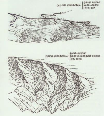
Introduction Meanwhile, theories of landscape evolution have grown in
nature and sophistication. As recently as the 1980s, the phrase
Geomorphology seeks to explain the diversity, origins and ‘landscape evolution model’ meant a word-picture describing
dynamics of terrain on the Earth and other planets. Our ability the sequential evolution of a landscape over geologic time
to do this rests on at least two basic pillars: quantitative char- (Figure 2A). William Morris Davis’ concept of the geographi-
acterization of terrain, and an ever-improving theory that cal cycle is a classic example of a conceptual landscape
describes the continual modification of topography by the evolution model. By the end of the 20th century, the term
many and varied processes that sculpt it. This paper reviews ‘landscape evolution model’ had taken on a new meaning: a
the state of the art in computational models of landscape mathematical theory describing how the actions of various
evolution, focusing on models that apply to terrain shaped by geomorphic processes drive (and are driven by) the evolution
a combination of fluvial and hillslope processes. of topography over time (Figure 2B). Typically, the governing
Since the late 1980s, our ability to measure topography has equations of landscape evolution are too complex to be solved
grown tremendously. As recently as the mid-1980s the vast in closed form and require a numerical solution method, and
majority of data on the Earth’s surface texture took the form for this reason ‘model’ has often come to refer to both the
of paper contour maps (Figure 1a). Large gaps in coverage underlying theory and the computer programs that calculate
existed and the task of quantifying the difference between one approximate solutions to the equations. The growing sophis-
landscape and another was a tedious and time-consuming tication in landscape models, as well as models for other
matter of extracting properties such as slope angles and drain- components of the Earth system, has prompted community-
age basin sizes from printed topographic maps or field surveys. wide modelling efforts such as the Community Surface
Twenty years later, digital elevation models now cover all of Dynamics Modeling System (CSDMS Working Group, 2004;
Earth’s landmasses between 60° north and south latitude at a CSDMS, 2008). The combined advances in computing and
resolution as fine as three arc seconds (~90 m) (Gesch et al., topographic data, together with advances in geochronology
2006), and in many countries, at a higher resolution. Moreover, (Bishop, 2007), have revolutionized our ability to measure
a small but rapidly growing fraction of the Earth’s surface has landforms and their rates of change, and to explore how these
been mapped by laser imaging technology at resolutions of forms and dynamics arise from the fundamental physics and
1 m or finer, and with very high accuracy (Figure 1b). chemistry of geomorphic processes.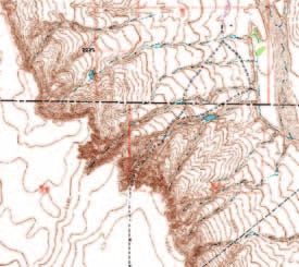
MODELLING LANDSCAPE EVOLUTION                                                                    29

                            (a)                                             (b)

Figure 1. Examples of topographic data, then and now. (a) Portion of a US Geological Survey 1:24 000 contour map for part of the West Bijou
Creek drainage basin, Colorado (Strasburg SE quadrangle). (b) Shaded relief image of the same area generated from a 1 m resolution (horizontal)
digital elevation model derived from Airborne Laser Swath Mapping data collected in April 2007 by the National Center for Airborne Laser Mapping
(NCALM). Images are approximately 3 km wide; north is up. This figure is available in colour online at www.interscience.wiley.com/journal/espl

 (A)                                                                         (B)

Figure 2. Landscape evolution models, then and now. (A) Conceptual sketch of stages in landscape evolution according to the model of W.M.
Davis, from the 4th edition of a popular geology textbook (Press and Siever, 1986). (B) Three frames from a numerical model of landscape evolu-
tion (CHILD; Tucker et al., 2001a), showing the development of topography and fan–delta complexes in response to vertical motion on a pair of
normal-fault blocks. The block toward the bottom in the images is subsiding relative to base level along the lower edge, while the block in the
background is rising. The shoreline position is shown by the heavy gray line. Lighter colours indicate higher altitudes, and vice versa. This figure
is available in colour online at www.interscience.wiley.com/journal/espl

Approach and scope                                                              The focus is on landscapes that are organized around drain-
                                                                             age basins and networks. Such ‘fluvial landscapes’ include
A number of excellent review papers have appeared in recent                  those in which the majority of sediment and solutes generated
years covering various aspects of geomorphic modelling.                      on hillslopes is transported away by running water in a drain-
However, although these offer a rich variety of perspectives                 age network. Landscapes that fall outside this definition
on the field, none provides a comprehensive introduction that                include eolian landscapes (arid regions in which most mass
covers the process ingredients, simplifications, and common                  transport is driven by wind), heavily karstified terrain (such as
algorithms that constitute the basic elements of numerical                   cockpit karst landscapes, in which most mass transport takes
landscape evolution models. This paper aims to fill this gap,                the form of groundwater transport of solutes; e.g. Lyew-Ayee
and thereby provide an entry point for geologists, geophysi-                 et al., 2007), ocean floors (where mass movement, density
cists, hydrologists, ecologists and others who wish to learn                 currents, and other processes dominate), and glacial terrain
more. We assume only an introductory-level knowledge of                      (in which the bulk of mass is transferred by moving ice). The
geomorphology, and that readers have a basic familiarity with                motivation for focusing on fluvial landscapes is not because
partial differential equations and related mathematical con-                 other landscapes are any less interesting, but simply because
cepts common to the physical sciences.                                       drainage basins and networks cover most the Earth’s land

Copyright © 2010 John Wiley & Sons, Ltd.                                                           Earth Surf. Process. Landforms, Vol. 35, 28–50 (2010)
                                                                                                                                       DOI: 10.1002/esp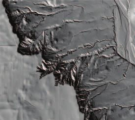
30                                                G.E. TUCKER AND G.R. HANCOCK

surface and because they have thus far received the most            Bishop, 2007). Regarding the erosion and transport rate laws
attention.                                                          that go into landscape models, Carson and Kirkby (1972)
   An area of considerable interest that is not examined at         discuss a variety of one-dimensional models of hillslope
length in this review is the application of landscape evolution     profile form and processes under different geomorphic sce-
theory and models. However, the issue of applications is            narios. Dietrich et al. (2003) provide an excellent recent
important enough to merit a few comments and some pointers          summary of rate laws for both hillslope and channel pro-
to relevant literature. Landscape evolution models serve a          cesses. Coulthard (2001) and Willgoose (2005) contrast the
number of roles in the science. First, they embody the com-         approaches of various model codes, and provide a valuable
munity’s latest ideas about how various physical and chemical       perspective on their strengths and weaknesses. Beaumont et
surface processes interact to shape Earth’s surface and transfer    al. (2000) discuss the coupling of geomorphic and tectonic
crustal mass from one place to another. Second, they allow          models. Other articles, such as Coulthard and Van De Weil
us to visualize and quantify the consequences of various            (2007), provide insight into the non-linear dynamics of land-
hypotheses about process dynamics. For many researchers,            scape evolution models. The edited monograph by Wilcock
the ability to visualize animated scenarios of landscape evolu-     and Iverson (2003) includes chapters on a wide range of topics
tion – even if they are purely hypothetical – provides a power-     related to geomorphic modelling, its scope and purpose,
ful stimulus to the imagination and enhances our ability to         approaches, and evaluation of models. Recent papers by
interpret the landscape. Likewise, numerical models make            Codilean et al. (2006) and Bishop (2007) are unique in that
quantitative, testable predictions about landforms and their        they link landscape evolution models, tectonics and topogra-
responses to various types of forcing. By revealing the logical     phy in an evaluation of the role that models and other tech-
consequences of our hypotheses, they direct our attention to        niques such as thermochronology can play in deepening our
those features of the landscape that provide the clearest tests     understanding of Earth surface processes.
of these hypotheses. Landscape evolution models have also              Papers and books dealing with general and philosophical
been widely used to develop insight into the geohistoric devel-     issues relevant to geomorphic modelling include Carson and
opment of particular places, from passive margins (Gilchrist        Kirkby (1972) and Kirkby (1996), who discuss the theoretical
et al., 1994; Kooi and Beaumont, 1994; Tucker and Slingerland,      underpinnings of the modelling approach used by many
1994; van der Beek and Braun, 1998) to compressional moun-          fluvial landscape evolution models, highlighting the role of
tain chains (Beaumont et al., 1992; Tucker and Slingerland,         models in the ‘dialogue between the development of theory
1996; Miller and Slingerland, 2007), among many others.             and the design of critical experiments’ (Kirkby, 1996, p. 262).
Bishop (2007) gives an overview of the role of numerical            Beven (1996) raises a note of caution concerning the potential
models, among other methods, in studies of long-term land-          for equifinality in geomorphic models. Oreskes et al. (1994)
scape evolution, while Beaumont et al. (2000) review coupled        provide a philosophical perspective on model structure and
models of tectonics and surface processes.                          issues surrounding verification and validation of not just land-
   Last but not least, landform evolution models can be used        scape evolution models but numerical models in general.
as management tools for the evaluation and rehabilitation of        Martin and Church (2004) provide a background to modelling
degraded landscapes, abandoned mines (Willgoose and Riley,          that focuses on the limitations of models and modelling
1998; Hancock, et al., 2000), contaminated sites, and land          approaches (echoing Oreskes et al., 1994) and provide new
development projects involving disturbance of soil and/or veg-      ideas on how these limitations can be mitigated.
etation (Coulthard and Macklin, 2003). They have been                  While all of the above work provides important back-
applied to problems of long-term hazardous waste manage-            ground, previous reviews have not simultaneously addressed
ment, such as the assessment of the likelihood that radioactive     the continuity frameworks, hydrologic approximations, geo-
wastes will remain encapsulated for periods as long as 10 000       morphic process ingredients, and algorithms that go into
years (Evans, 2000). The modelling of landscape evolution           numerical landscape models. This paper attempts to fill this
and soil erosion thus has important environmental                   gap by providing an overview of landscape development
applications. Modelling allows for idea testing, evaluation of      process laws, including continuity of mass, geomorphic trans-
different surface material properties, and analyses of risk         port functions, and numerical methods for solving the consti-
(Oreskes et al., 1994).                                             tutive equations with an eye on the strengths and limitations
   Because landscape evolution models allow the landscape           of the different approaches. We begin with a brief history of
surface to change through time both in elevation and in terms       models, and then turn to an examination of the common
of catchment size and shape, they can be used to address            process ingredients.
dynamic phenomena such as gully network development
and valley alluviation, which is generally not possible with
fixed-terrain models such as the USLE and RUSLE (Hancock,           Brief History of Landscape Evolution Models
2004). They also offer the advantage that the terrain can be
evaluated visually as it develops through time. Landscape           Early roots of landscape evolution theory can be found in the
evolution models have been used for problems ranging from           writing of the renowned 19th century geologist Grove Karl
short-term soil loss assessment (i.e. tonnes per hectare per        Gilbert. In his remarkable monograph on the Henry Mountains
year) and the processes causing soil loss (e.g. rill or interrill   of Utah, USA, Gilbert (1877) outlined a group of hypotheses,
erosion) along single hillslopes (Hancock et al., 2007) through     in the form of word-pictures, to describe how the mechanics
to catchment-scale assessments over geologic time (104–106          of weathering, erosion, and sediment transport lead to the
years) (Hancock et al., 2008a). Nevertheless, the evaluation        genesis of various landforms. In retrospect, it seems an obvious
and refinement of landform evolution models is very much            next step to translate these word pictures into equations, but
ongoing.                                                            several decades elapsed before this began to happen. In a
   There have been numerous reviews of landscape evolution          series of papers, Culling (1960, 1963, 1965) explored the
models and modelling approach in geomorphology (Carson              morphologic consequences of Gilbert’s hypothesis that the
and Kirkby, 1972; Kirkby, 1996; Coulthard, 2001; Bras et al.,       average rate of downslope sediment flux on hillslopes depends
2003; Wilcock and Iverson, 2003; Martin and Church, 2004;           on the local gradient. This hypothesis leads to the following
Whipple, 2004; Willgoose, 2005; Codilean et al., 2006;              flux equation (written here in one dimension):

Copyright © 2010 John Wiley & Sons, Ltd.                                                Earth Surf. Process. Landforms, Vol. 35, 28–50 (2010)
                                                                                                                            DOI: 10.1002/esp
MODELLING LANDSCAPE EVOLUTION 31
Table I. Partial list of numerical landscape evolution models published between 1991 and 2005
a
Model Example reference Notes
SIBERIA Willgoose et al. (1991) Transport-limited; introduces channel activator function
DRAINAL Beaumont et al. (1992) Fluvial transport based on ‘undercapacity’ concept
GILBERT Chase (1992) Cellular automaton
DELIM Howard (1994) Detachment-limited
GOLEM Tucker and Slingerland (1994) Introduces algorithms for regolith generation and landsliding
CASCADE Braun and Sambridge (1997) Introduces irregular discretization method
CAESAR Coulthard et al. (1997) Cellular automaton algorithm for 2D flow field
ZSCAPE Densmore et al. (1998) Introduces stochastic bedrock landsliding algorithm
CHILD Tucker and Bras (2000) Introduces stochastic treatment of rainfall and runoff
€ROS Crave and Davy (2001) Modified precipiton algorithm
APERO/CIDRE Carretier and Lucazeau (2005) Single or multiple flow directions
a
First reference in mainstream literature.
∂η the initial and boundary conditions on the system (including
qs = −Kc (1) climate forcing, baselevel controls, and substrate representa-
∂x
tion); our treatment of these is embedded in the discussion of
Here, qs represents the average volumetric sediment transport the five components listed above. Each of these components
rate per unit slope width, η is land-surface elevation, x is will be reviewed in turn, followed by consideration of some
distance down slope, and Kc is a rate coefficient that depends general issues and challenges.
on process, climate, and material. Equation (1) is an example
of a geomorphic transport law, which Dietrich et al. (2003)
define as ‘a mathematical expression of mass flux or erosion Continuity of mass
caused by one or more processes acting over geomorphically
significant spatial and temporal scales’. (In order to distinguish At first glance, the issue of mass continuity seems trivial.
these from fundamental principles such as the Ideal Gas Law, Geomorphic systems, whatever their complexity, involve
we will refer to them here as geomorphic transport functions, neither relativistic speeds nor nuclear reactions, and therefore
or ‘GTFs’.) When combined with an equation of mass continu- mass is conserved absolutely. However, there are a number
ity (discussed below), GTFs describe the evolution of topog- of different possible frameworks for mass conservation in a
raphy over time under the action of particular processes. geomorphic system, and each has its own assumptions and
From the early 1960s onward, a series of GTFs for hillslope limitations. In fact, the choice of a framework for mass conti-
processes were introduced. These new (and often purely nuity dictates the type of processes and circumstances that can
hypothetical) GTFs described processes ranging from slope be addressed, so it is worth taking some time to review the
wash to chemical erosion and soil development; many of the pros and cons of some common continuity expressions.
early ones are summarized in Carson and Kirkby (1972). By The most general statement of mass continuity for a control
the 1970s, researchers had begun exploring models of three- volume V is, in words:
dimensional slope forms (Ahnert, 1976; Hirano, 1976;
Armstrong, 1976). time rate of change in mass in control volume = mass rate
From the 1990s onward, as computers continued to get in – mass rate out
faster, numerical models of fluvial landscape evolution con-
tinued to grow in number and in sophistication. A partial list The right-hand side represents processes; the left represents
of current models appears in Table I. These computer codes the nature and geometry of the idealized model system. The
encompass a wide variety of GTFs for channels and hillslopes, most common continuity expressions in geomorphic models
and employ a range of solution methods. Reviews and com- begin with a thin vertical column of rock and/or soil (or more
parisons of recent models are given by Coulthard (2001) and generally, regolith) (Figure 3A). The column has horizontal
Willgoose (2005). In this paper, our aim is not so much to dimensions dx by dy, and the height of the land surface rela-
compare model codes and formulations, but rather to familiar- tive to a datum that represents baselevel (such as sea level) is
ize the reader with the conceptual and mathematical bases for denoted by the symbol η. Mass balance dictates that
landscape evolution models and to highlight some unresolved
issues and current research needs. ∂ρη
= ρsrcB − ∇ ( ρsqs ) (2)
∂t
Model Components where t is time, qs is a transport-rate vector (volumetric trans-
port rate per unit time per unit width in a particular direction),
A landscape evolution model contains several components: B [L/T] is a source term (such as uplift or subsidence relative
(1) a statement of continuity of mass; (2) geomorphic transport to a given baselevel, or direct accumulation by eolian sedi-
functions that describe the generation and movement of sedi- ment input, etc.), and ∇ is the divergence operator, in this case
ment and solutes on hillslopes; (3) a representation of runoff representing divergence in two spatial dimensions (∇u = ∂ux/∂x
generation and the routing of water across the landscape; (4) + ∂uy/∂y, where ux and uy are the x and y components of the
geomorphic transport functions for erosion and transport by vector u). Each term in Equation (2) has dimensions of mass
water and water-sediment mixtures (Dietrich et al., 2003); and flux per time per unit surface area. The three densities are as
finally (5) numerical methods used to discretize the solution follows: ρ = average density of rock/sediment/soil in the
space and iterate forward in time to obtain approximate solu- column, ρsrc = density of input source material (its value
tions to the governing equations. Other considerations include depends on what the source term is meant to represent; for
Copyright © 2010 John Wiley & Sons, Ltd. Earth Surf. Process. Landforms, Vol. 35, 28–50 (2010)
DOI: 10.1002/esp32 G.E. TUCKER AND G.R. HANCOCK
(A) (B) ∂H 1
= (Ps − ∇qs ) (4a)
∂t 1− φ
∂R
η H
SOIL = B − Ps (4b)
∂t
η =R+H (4c)
R
SOIL ROCK
or Here, R is the altitude of the bedrock–regolith contact, and Ps
ROCK represents the rate of conversion of rock to soil in terms of
equivalent rock thickness per unit time (Ahnert, 1976, 1987;
Dietrich et al., 1995; Heimsath et al., 1997, 2000).
The majority of landscape evolution models use either
dy dy Equation (3) or (4), with varying representations of the process
dx dx terms. What goes into the process terms will be discussed in
the next section. Before moving on to look at rate laws for Ps
Figure 3. Two control volumes for continuity of mass. (A) Uniform and qs, it is important to note that the vertical-column continu-
substrate. (B) Division between regolith (or soil) and bedrock, with a ity Equations (3) and (4) are simplistic. There are quite a few
regolith layer of time- and space-varying thickness. landforms that do not fit into this framework, including those
with vertical or overhanging faces (such as cliffs, waterfalls,
gully headscarps, cut banks, and tafoni). To some extent these
can be handled by simply using horizontal rather than vertical
columns (Kirkby, 1984, 1992; Howard, 1998), though
instance, if B represents uplift of rock relative to the geoid, this method seems to be practical only for modelling one-
then ρsrc is the density of rock entering through the base of the dimensional landforms, such as cliff profiles, in isolation.
column), and ρs = the bulk density of sediment and/or solutes Another limitation of the popular two-dimensional continu-
entering and leaving the sides of the column (which includes ity frameworks is their inability to represent vertical variations
sediment flowing in and out, at or near the land surface). in weathering rates, shallow groundwater flow, and regolith/
Equation (2) is quite general because it allows for dynamic rock properties. To do this properly requires a three-
changes in density throughout the column, for example due dimensional approach: subdividing columns vertically, and
to iso-volumetric conversion of bedrock to saprolite. In order specifying equations to represent the vertical variation in soil
to make Equation (2) useful, however, the density distribution properties (composition, porosity, mineral density, etc.; see for
within the column needs to be specified. One common and example Kirkby’s (1976) soil-deficit concept) as well as verti-
simple approach is to assume that the column consists almost cal fluxes of mass due to soil strain (e.g. gravitational compac-
entirely of rock, with a thin soil or sediment layer near the tion; contraction/expansion due to changes in mineralogy; e.g.
surface, so that average column density is effectively equal to Brimhall and Dietrich, 1987) and the advection of soil layers
rock density, ρr. If one assumes that the sediment-grain density toward (or away from) the eroding (or aggrading) land surface.
Ps equals the rock density Pb, and that B represents rock uplift It is important also to bear in mind that Equations (3) and (4)
(so Psrc = Pr), Equation (2) simplifies to are designed around processes that can be considered as flows
or currents of mass, rather than as events. This will be revisited
∂η below.
= B − ∇q s (3)
∂t
Alternatively, one could assume that the entire column consists
of regolith that has uniform porosity, φ, and grain density, in Geomorphic transport functions for
which case the resulting continuity equation is the same as (3) hillslope processes
but with the multiplier 1/(1−φ) in front of the right-hand term.
Equation (3) and the assumptions behind it are commonly Geomorphic transport functions represent the theoretical core
used in landform evolution models. It is important to bear in of a landscape evolution model. Dietrich et al. (2003) provide
mind its limitations, however. First, surface height, η, is a thoughtful review of the nature, purpose, and current status
assumed to be a single-valued function of horizontal position of GTFs. In this section, we review the strengths and weak-
(x,y), which makes it impossible to represent vertical faces and nesses of current GTFs for hillslope processes, including rock
overhangs. Second, variations in height due to compaction or disintegration and regolith generation, together with mass
expansion of underlying soil are ignored (this would be inap- movement and landsliding.
propriate, for example, in highly soluble rock). Third, Equation
(3) does not allow for variations in the thickness or properties Rock disintegration and regolith generation
of the soil (or regolith) layer, and thereby ignores effects such On its way to the Earth’s surface, rock particles pass through
as the potential dependence of sediment transport rate on what has come to be called the ‘critical zone,’ defined as ‘the
regolith thickness (Carson and Kirkby, 1972; Anderson and layer bounded by the top of the forest canopy and the base of
Humphrey, 1989; Kirkby, 1992; Braun et al., 2001), and the weathering horizon’ (National Research Council, 2001).
potential feedbacks between soil water storage capacity, A complete theory of landscape evolution must ultimately
runoff generation, weathering, and sediment transport (Kirkby, include a description of how processes in the critical zone
1976; Saco et al., 2006). weaken rock through fracturing, mechanical wedging, chemi-
A somewhat more sophisticated approach, which takes cal alteration, biological disruption and mixing, and so on.
account of variations in regolith thickness, starts from the However, although most textbooks contain a long list of physi-
assumption that there is an abrupt contact between loose, cal and chemical weathering processes, it is only recently that
mobile regolith, with thickness H and uniform density ρsoil, the research community has begun to develop and test
and the underlying rock (Figure 3B): mathematical models to predict rates and patterns of rock
Copyright © 2010 John Wiley & Sons, Ltd. Earth Surf. Process. Landforms, Vol. 35, 28–50 (2010)
DOI: 10.1002/espMODELLING LANDSCAPE EVOLUTION 33
disintegration by specific chemical and physical processes ics and chemistry of weathering processes is needed in order
(Fletcher et al., 2006; Cohen et al., 2009). to determine mathematical functions that relate rates of rock
Current theory for regolith production builds on Gilbert’s disintegration to factors such as subsurface temperature history
(1877) hypothesis that the rate of rock disintegration varies (Walder and Hallet, 1985; Anderson, 1998), state of stress
inversely with the thickness of the overlying regolith mantle. (Miller and Dunne, 1996; Molnar, 2004), and rates of mineral
This was expressed by Ahnert (1967) in the form of an expo- alteration (Fletcher et al., 2006; Wells et al., 2006).
nential decay function:
Mass movement and landsliding
Ps = Ps0 exp( −H H* ) (5) Gravity-driven mass movement takes on a wide variety of
forms, with characteristic time scales ranging from a few
where the two parameters are Ps0, the rate of regolith produc- seconds (e.g. rockfall) to tens or hundreds of millennia (e.g.
tion from bare bedrock (rock thickness converted per unit soil creep; Fernandes and Dietrich, 1997). A linear slope-
time) and H*, a characteristic decay length scale. The expo- dependent transport function has been widely used to model
nential form is chosen simply because it smoothly varies from soil creep on relatively low-gradient (> H*). processes, including soil displacement by plants and animals,
Equation (5) is purely heuristic, with no physical or chemi- expansion and contraction due to freeze–thaw or wet–dry
cal basis in any particular process, but it does make testable cycling, and dispersion by raindrop impact on bare soil,
predictions. The exponential decay function implies that, all among others. What sets these processes apart from landslid-
else being equal (i.e. constant Ps0 and H*), under steady condi- ing is the short length scales of individual displacement events
tions – in which the thickness of the regolith changes slowly (we will revisit this distinction below).
relative to the rate of surface erosion – one should see an The linear creep function
inverse relationship between regolith thickness and erosion
rate. This prediction has been tested in several field cases, qs = −Kc∇η, (7)
using cosmogenic nuclide measurements at the bedrock–soil
contact to measure average erosion rates (McKean et al., 1993; where Kc is a constant, is the most widely used and tested
Heimsath et al., 1997, 2001; Small et al., 1999), and it turns geomorphic transport function. It accounts for convex-upward
out to be consistent with observations in settings ranging from hillslope profiles, and has been tested and calibrated using
semi-arid coastal mountains to high alpine terrain. cosmogenic nuclide mass-balance measurements (McKean et
One might reason, as did Gilbert, that weathering processes al., 1993; Heimsath et al., 1997, 2001, 2005; Small et al.,
involving water should reach their maximum efficiency under 1999). The creep function has been widely applied to scarp
a finite regolith thickness: deep enough to trap and hold water degradation, including fault scarps and fluvial, marine, and
against the rock, but shallow enough that the rock surface is lake-shore terraces (Colman and Watson, 1983; Hanks et al.,
not strongly insulated against temperature swings, frequent 1984; Andrews and Hanks, 1985; Andrews and Bucknam,
water flushing, plant and animal activity, etc. Several different 1987; Avouac, 1993; Avouac and Peltzer, 1993; Rosenbloom
mathematical forms have been suggested (Ahnert, 1976; Cox, and Anderson, 1994; Arrowsmith and Rhodes, 1994; Enzel et
1980); an example is Anderson’s (2002) approach: al., 1996; Arrowsmith et al., 1998; Niviere et al., 1998; Hanks,
2000; Font et al., 2002; Phillips et al., 2003; Hsu and Pelletier,
Ps = min [Ps0 + bH , Ps1 exp ( −H H* )] (6) 2004; Kokkalas and Koukouvelas, 2005; Nash and Beaujon,
2006; Pelletier et al., 2006). Estimates of the rate coefficient
where Ps0 is the bare-bedrock production rate, b scales the Kc have been obtained from a variety of approaches (see
rate of increase in production rate with thickness, and Ps1 sets compilation by Martin and Church, 1997). Although some
the intercept of the exponential decay. This ‘humped curve’ progress has been made in deriving either the form or value
implies a runaway feedback. When regolith cover falls below of Kc for particular processes (Kirkby, 1971; Carson and Kirkby,
a critical thickness, the production rate slows, which promotes 1972; Black and Montgomery, 1991; Anderson, 2002; Gabet,
further thinning and leads ultimately to bedrock exposure at 2000; Furbish et al., 2007), for many processes Kc is treated
the surface. It has been suggested that this mechanism can as an empirical parameter.
lead to the formation of tors and inselbergs (Ahnert, 1987; Although Kc is usually assumed constant, physical consid-
Anderson, 2002; Heimsath, et al., 2001; Strudley et al., 2006). erations dictate that it must have some degree of dependence
Saco et al. (2006) generalized the exponential decay rule to on regolith thickness; if nothing else, the creep rate should
include the spatial distribution of soil moisture and modelled vanish as regolith thickness approaches zero, regardless of
realistic patterns of hillslope scale bedrock etching and spatial slope angle. Several depth-dependent creep functions have
distribution of soil depth. been suggested (Ahnert, 1976), ranging from a simple ‘on-off
Kirkby (1976, 1985) developed an interesting alternative to switch’ (Rosenbloom and Anderson, 1994) to models based
the exponential-decay models. Instead of assuming a sharp on process mechanics (Kirkby, 1971; Carson and Kirkby,
contact between bedrock and regolith, Kirkby’s approach 1972; Anderson, 2002) or a hypothesized similarity to fluid
describes the transition from rock to regolith as a gradational flow (Braun et al., 2001). What is needed now is (a) more
process in which the state variable is the ‘soil deficit,’ repre- process-specific models for Kc, and (b) field and experimental
senting the fraction of intact (unweathered) rock remaining at tests of these models.
a particular level in the soil profile. The soil-deficit approach From studies of scarp degradation (see references above),
is more appropriate for situations that have a wide interface biogenic transport (Gabet, 2000; Heimsath et al., 2001), hill-
zone between unaltered parent material and fully weathered, slope morphology (Roering et al., 1999), sediment yield
mobile soil. (Martin, 2003), and experimental sand piles (Roering, 2004),
The success of the exponential-decay rules in explaining it is clear that the linear creep function underpredicts transport
observed regolith-thickness patterns is encouraging, but there rates on gradients that are near the angle of repose for natural
remains a need to develop a physico-chemical process basis soils. This has motivated the development of several nonlinear
for the embedded parameters. Further research on the mechan- transport functions that allow transport rates on steep slopes
Copyright © 2010 John Wiley & Sons, Ltd. Earth Surf. Process. Landforms, Vol. 35, 28–50 (2010)
DOI: 10.1002/esp34 G.E. TUCKER AND G.R. HANCOCK
to increase at a greater-than-linear rate with gradient (Anderson flux-function approach to shallow landsliding is that it incor-
and Humphrey, 1989; Howard, 1994; Roering et al., 1999; porates time averaging and therefore describes sediment trans-
Gabet, 2000). For example, Howard (1994) explored the port rates on time scales relevant to landform evolution. The
transport function chief drawback is the assumption of locality: flux at a point
depends only on local variables (such as slope angle), irre-
KD ∇η spective of the particular trajectory and momentum of any
qs = (8)
1− ( ∇η Sc )a particular flow. Tucker and Bradley (in press) explore the
limitations of the locality assumption in hillslope transport
where Sc is a threshold gradient that represents the point of theory using a particle-based model that illustrates the mor-
mechanical failure. The formula was intended particularly for phological significance of long-distance transport events on
transport by numerous small, shallows slide events. At small steep slopes. In principle, long-distance transport effects could
gradients, this nonlinear transport function is close to the be parameterized based on expected flow paths, perhaps
linear model (Equation (7)), while as gradient approaches the using insights derived from laboratory or computer experi-
threshold from below, the transport rate approaches infinity. ments on the net effect of many landslides. To the best of our
Equation (8) (with a = 2) is consistent with creep behaviour in knowledge such an analysis has not yet been attempted,
experimental sand piles (Roering, 2004) and with 3D slope though recent models of debris-flow routing (Benda and
forms obtained from high-resolution altimetry (Roering et al., Dunne, 1997; Stock and Dietrich, 2003, 2006) do use infor-
1999, 2008). In principle the parameter Sc represents the mation about upstream topography in estimating the average
threshold failure gradient for shallow soil, and so could be sediment flux at a point downstream. Similarly, Foufoula-
estimated using standard geotechnical methods. Georgiou et al. (in press) and Furbish and Haff (in review) have
Transport functions for other types of mass movement – developed continuum formulations that acknowledge long-
shallow and deep landsliding, rockfall, rotational slides, distance transport events, using (respectively) a fractional dif-
slumps, etc. – are more problematic. For slow but deep-seated fusion and a Fokker–Planck approach.
mass movements such as rotational slumps, particle displace- An alternative approach is to explicitly model the initiation
ment during a motion event may typically be small relative to of individual landsliding events and track their motion across
the length of a hillslope, but the depth to the failure plane may topography. Densmore et al. (1998) used a Lagrangian method
be a significant fraction of the hillslope relief. The standard to model bedrock landsliding in the ZSCAPE model, using a
continuity framework (Equations (3) and (4)), which is designed stochastic triggering algorithm, while van der Beek and Braun
for near-surface sediment transport, is ill-equipped to handle (1998) introduced a similar approach to model landsliding in
deep-seated motion. A more appropriate continuity equation the CASCADE landscape evolution model. Lancaster et al.
for deep-seated landslides might have the form: (2003) use an event-based, momentum-balance approach to
model erosion and sedimentation by debris flows in a modi-
∂η fied version of the CHILD model (Tucker et al., 2001a).
= −∇ ( v l h) (9)
∂t Howard (1998) developed a 1D model of gully formation on
Mars using a Lagrangian approach to track the motion of
where the vector vl is the horizontal velocity of the landslide individual landslides. A simpler variation on this theme was
mass, and h is depth to the failure plane (note that this expres- used by Tucker and Slingerland (1994) and Tucker and Bras
sion ignores rotation, but it does allow for spatial variation in (1998) to impose an upper limit to slope angle while maintain-
the velocity and thickness of the slump mass). To date, deep- ing continuity of mass. The advantage of these various event-
seated landsliding has not been explicitly incorporated in a based approaches is that they take advantage of current
landscape evolution model. knowledge of landslide triggering and motion, while the main
Shallow, rapid landsliding presents a different sort of chal- disadvantage is the loss of computational efficiency. In a
lenge. The standard 2D continuity framework is built on the similar vein, particle-based models of hillslope transport
concept of near-surface flows of sediment that add or subtract (Jyotsna and Haff, 1993; Tucker and Bradley, in press) provide
mass at the top of a rock/sediment column. A shallow land- a link between transport statistics, topography, and morpho-
slide, by definition, is one in which the depth of failure is small logic evolution.
relative to hillslope relief, and in that sense shallow landslid-
ing fits the concept of near-surface transport. However, the
standard continuity framework is also based on the idea that Flowing water: the St. Venant equations and
transport of sediment grains can be treated in the same manner various approximations
as heat or fluid transport: as long as the space and time scales
for individual particle motions are small relative to the scales A large fraction of geomorphic work in a drainage basin is
of interest, transport can be represented as a time-averaged accomplished by running water, so the treatment of runoff
continuum flux (Tucker and Bradley, in press). With shallow dynamics is a central issue in landscape evolution models.
landsliding, the event times are suitably short, but the dis- This section reviews various methods that landscape evolution
placement length scales are commonly a large fraction of models typically use to represent the flow of water over (and
hillslope length. This raises some challenges in formulating sometimes beneath) the land surface. Because many models
GTFs for shallow landsliding, as well as for dry ravel (Gabet, use cellular algorithms to compute the routing of water across
2003), which also involves long-distance motion events. terrain, this section also includes a discussion of spatial dis-
Two general approaches have been used to handle rela- cretization methods. A common theme behind all of the
tively shallow, rapid landsliding in landscape evolution various flow-routing methods is the need to reconcile the very
models: flux-based models and event-based models. Flux- short characteristic time scales (minutes to seasons) associated
based models of shallow landsliding are intended to approxi- with hydrologic processes with the much longer time scales
mate a natural series of events in terms of the resulting (decades to epochs) associated with landform change.
long-term average rate of mass transfer from point to point, In the 2D world implied by standard continuity frameworks,
using a transport function of the form qs = f (topography, mate- we turn to the St. Venant or shallow-water equations as a
rial, climate, etc.) (Kirkby, 1987). A key advantage of the starting point. The St. Venant equations are the vertically
Copyright © 2010 John Wiley & Sons, Ltd. Earth Surf. Process. Landforms, Vol. 35, 28–50 (2010)
DOI: 10.1002/espMODELLING LANDSCAPE EVOLUTION 35
Table II. The St. Venant or shallow-water equations
Equation number Equation Notes
T1 ∂h ⎛ ∂uh ∂vh ⎞ Continuity of mass; i = input precipitation minus losses,
= i −⎜ + ⎟
∂t ⎝ ∂x ∂y ⎠ h = flow depth
T2* ∂uh ∂ ∂ ∂h ∂η τ bx Continuity of momentum, x-direction; u and v = x- and y-directed
+ (hu 2 ) + ( huv ) + gh + gh + =0
∂t ∂x ∂y ∂x ∂x ρ velocity, τb = boundary shear stress, ρ = water density
T3* ∂vh ∂ ∂ ∂h ∂η τ by Continuity of momentum, y-direction
+ (hv 2 ) + (huv ) + gh + gh + =0
∂t ∂y ∂x ∂y ∂y ρ
T4 τbx = Cfρu|u|, τby = Cfρv|v| Friction; Cf = dimensionless friction factor
* The terms in T2 and T3 represent, from left to right: local acceleration, streamwise inertia, cross-stream inertia, pressure, gravity, and friction.
Dropping local acceleration gives the gradually varied flow equations. Dropping local acceleration and inertia gives the diffusion wave
approximation. Dropping these plus the water-depth (pressure) gradient gives the kinematic wave approximation.
integrated form of the Navier–Stokes equations for incom- where ρ is fluid density (water plus any sediment), q is dis-
pressible, free-surface flow. They contain four parts (Table II): charge per unit width in the direction of flow, S0 is bed slope
continuity of mass (T1), continuity of momentum in two hori- (also in the direction of flow), and Cf is a dimensionless friction
zontal dimensions (T2 and T3), and a friction function that coefficient. For fully rough (turbulent) flow, Cf has a weak
describes the relation between flow resistance and fluid veloc- dependence on flow depth; for laminar or transitional flow, it
ity (T4). If the shallow-water equations were easy to solve depends on the Reynolds number (see, for example, Furbish,
analytically or numerically, one would expect to find these 1996).
equations in their full form in every drainage-basin evolution
model. Unfortunately, they are not: there is no known analyti- Cell-based routing schemes
cal solution to the full equations, and numerical solutions are The 2D kinematic wave approximation implies that flow lines
both tricky to implement and computationally expensive. always follow topography. Many landscape evolution models
Thus, when one meets these fluid flow equations in a land- take this one step further by using a cellular routing algorithm:
scape evolution model, they have often been considerably all water leaving a cell flows to whichever of the adjacent cells
simplified. In this section, the various simplified forms of the lies in the direction of steepest descent. At this point, it is
shallow-water equations are reviewed, so that the reader has useful to digress briefly and look at how numerical landscape
a guide to the type of simplifications that are typically made evolution models represent topography, because the cellular
in landscape evolution models and the limitations that these routing algorithms are fundamentally linked to the spatial
imply (Singh, 2001). More about the St. Venant equations and discretisation scheme.
their simplified forms can be found in most hydrology text- The equations of water and sediment motion, whatever their
books (e.g. Streeter and Wylie, 1981). particular forms, require a numerical solution method in
Before looking at simplified forms, it is important to recog- which the continuous landscape surface is divided into dis-
nize the four basic forces driving fluid flow in equations T2 crete elements. Many models use a lattice of square cells,
and T3: inertia, gravity, fluid pressure, and boundary friction. which lends itself to finite-difference solutions but can be
A common simplification is to assume quasi-steady flow (neg- somewhat inflexible (Figure 4a). The CASCADE and CHILD
ligible acceleration/deceleration in time), so that the time models use an irregular discretization in which nodes are
derivative on the left-hand side of T2 and T3 goes to zero; the connected by a Delaunay triangulation and the surface area
resulting simplification is known as the gradually varied flow of each node is represented by a Voronoi (or Thiessen) polygon
approximation. Many overland and channelized flows accel- (Braun and Sambridge, 1997; Tucker et al., 2001a,b) (Figures
erate only slowly in space (at least when velocity is considered 4 and 5). Both models use a finite-volume solution method
at the reach scale), and this motivates the common practice that tracks fluxes across cell boundaries. Simpson and
of neglecting the inertial terms in T2 and T3. Dropping both Schlunegger (2003) developed a model that uses triangular
the time derivative and the inertial terms yields the diffusion- elements in a finite-element solution to the flow and transport
wave approximation, which applies to flows that are driven equations.
mainly by gravity and pressure gradients; the latter arise from On a regular lattice, the steepest-direction routing method
variations in flow depth along a streamline. When the rate of is identical to the ‘D8’ algorithm commonly used to route
change of flow depth with distance along a slope or channel water across digital elevation models (Figure 4a); the approach
is small relative to the bed surface slope, the flow will be is easily adapted to an irregular Voronoi mesh (Figure 4b)
driven primarily by gravitational pull. For such flows, one can (Tucker et al, 2001b). The advantages of the cell-routing
omit the pressure-gradient term in T2 and T3 to obtain the approach are simplicity and speed. One weakness is the lack
well known kinematic wave equations, in which acceleration of ability to handle diverging flow. Another is the problem of
of water by Earth’s gravitational pull is everywhere exactly kinematic flow convergence noted later. In practice, the width
balanced by friction. With a little bit of algebra, one can see of flow is either assumed equal to grid-cell width (Willgoose
that, for gravity-driven (kinematic) flows, the local bed shear et al., 1991a), which leads to a grid-size dependence in flow
stress, averaged over a flow-perpendicular cross-section, is depth and velocity. Alternatively, flow is assumed to be con-
simply fined to a sub-grid-cell channel feature (Howard, 1994; Tucker
and Slingerland, 1996), the width of which is specified empiri-
τ 0 = ρ ghS0 = ρ g 2/3Cf 1/3q2/3S0 2/3 (10) cally (more on this below).
Copyright © 2010 John Wiley & Sons, Ltd. Earth Surf. Process. Landforms, Vol. 35, 28–50 (2010)
DOI: 10.1002/esp36 G.E. TUCKER AND G.R. HANCOCK
The single-flow-direction assumption has been relaxed in Qi Siα
=
some models by either encoding an explicit numerical solu- Qtotal N
(11)
tion to the steady 2D kinematic wave equations for steady ∑S
i =1
α
i
flow (Simpson and Schlunegger, 2003) or using a multiple-
direction algorithm in which outgoing flow from a cell is split
among one or more downslope neighbours, weighted accord- where Qtotal is the total discharge of water flowing through the
ing to gradient in each direction: grid cell, Qi is the discharge of water into the immediate
downstream cell i, N represents the number of neighbouring
cells that are lower than the origin cell, and α is a parameter.
The value α = ½ can be derived from a simple kinematic
momentum-balance argument (Murray and Paola, 1997). Use
(a) of a multiple-direction scheme provides a better description
of overland flow on convex hillslopes and fans (Moglen and
Bras, 1994; Pelletier, 2004).
Murray and Paola (1994, 1997) created a cellular, multiple-
flow direction algorithm to model flow and sediment transport
in a river channel. Their approach involves a form of multiple-
flow-direction algorithm similar to Equation (11), using three
potential downstream flow directions at each node and allow-
ing for uphill flow (negative slopes in Equation (11)) when all
three downstream directions have positive gradients. Their
approach was generalized to handle all possible flow direc-
tions, and to incorporate water depth, in the CAESAR model
by Coulthard et al. (1999, 2002). Both algorithms provide an
efficient means of approximating a time-varying, two-dimen-
sional flow field without the expense of a traditional numerical
solution to the shallow-water equations.
Spatially variable and non-steady flow models
Most landscape evolution models that use cell-based or kine-
matic-wave water routing also assume steady flow (the rate of
outflow at any point equals incoming rainfall minus any
losses). The SIBERIA and DELIM models treat discharge (Q) as
(b) a power function of drainage area (A), Q = Kq Amq , although in
practice mq (constant) is often set to unity with Kq a constant
(Willgoose et al., 1991a; Howard, 1994), which implies runoff
in equilibrium with steady, uniform rainfall. Sólyom and
Tucker (2004) explored the consequences of non-equilibrium
runoff using a simple model that relates peak discharge to the
ratio of storm duration and basin concentration time, and
demonstrated the potential for significant (and scale-depen-
dent) geomorphic effects. Effects of spatially variable runoff
generation have also been encoded and explored in some
drainage network evolution models. One finding is that satu-
ration-excess runoff generation tends to enhance hillslope
convexity and hillslope-channel transitions in equilibrium
landscapes (Ijjasz-Vasquez et al., 1992; Tucker and Bras,
1998). In fact, there are many fascinating and unanswered
Figure 4. Schematic illustration of cell-based, single-flow-direction questions regarding the feedbacks between climate, hydrology
routing schemes. (a) Regular grid. (b) Voronoi mesh. (Modified from and landscape evolution. While models of drainage basin
Tucker and Slingerland, 1994 and Tucker, 2004, respectively.) evolution have begun to address some of these, including
Figure 5. Drainage network response to a step increase in the rate of baselevel fall. Shading indicates boundary shear stress (light = high, dark
= low). (A) Detachment-limited model. (B) Transport-limited model. Both models include a threshold for erosion/transport and a stochastic
sequence of rainstorm events.
Copyright © 2010 John Wiley & Sons, Ltd. Earth Surf. Process. Landforms, Vol. 35, 28–50 (2010)
DOI: 10.1002/espMODELLING LANDSCAPE EVOLUTION 37
issues of both precipitation distribution and phase (Beaumont with a ‘geomorphically effective’ runoff event. The concept
et al., 1992; Roe et al., 2002; Anders et al., 2008) as well as involves using a single, steady runoff coefficient that is pre-
runoff generation (Sólyom and Tucker, 2004; Huang and sumed to be equivalent, in terms of geomorphic effectiveness,
Niemann, 2006), the topography-hydrology-climate connec- to a natural series of runoff events. Willgoose et al. (1989)
tion remains a rich problem to be explored. justified this approach by deriving a time-averaged sediment
transport equation based on the Einstein–Brown formula (see
Diffusion-wave routing models Julien (1998)) in which the applicable discharge is the mean
Kinematic-wave theory provides a good approximation for a annual peak discharge; however, because some terms were
wide range of overland and channelized flows (see Singh discarded, the result is approximate rather than exact unless
(2001) for a review). From the viewpoint of landscape evolu- the discharge exponent is an integer. Huang and Niemann
tion, however, there is at least one important weakness. As (2006) analysed the return period of the geomorphically effec-
Izumi and Parker (1995) noted, in locations where overland tive event under a range of erosion laws and catchment states,
flow converges – such the axis of a valley – a purely kinematic and found that in general the event return period – and thus
assumption predicts infinitely narrow, infinitely deep flow, its intensity – varied systematically throughout the network in
because the pressure (depth) gradient that would normally most cases.
prevent this is omitted. Thus, while the kinematic approxima- Several studies have explored the role of discharge vari-
tion works well for many 1D flows, applying it in two dimen- ability in time (Willgoose, 1989; Tucker and Bras, 2000;
sions requires a means of ensuring a finite flow width along Molnar, 2001; Tucker, 2004; Molnar et al., 2006; Lague et al,
lines of terrain convergence. The problem of flow conver- 2005). Though the details vary, a common conclusion among
gence along valley axes presents an obstacle to properly cap- these studies is that, all else being equal, erosion and transport
turing the transition from distributed (sheet wash) to rates will tend to increase when discharge fluctuates more
concentrated (channelized) flow. Although landscape models strongly over time, simply because erosion and transport rates
that assume purely slope-driven (kinematic) runoff can produce tend to depend more-than-linearly on discharge. Tucker and
forms that resemble hillslopes and channels, the hillslope– Bras (2000) implemented stochastic rainfall and runoff in a
channel transition point often depends on model resolution landscape evolution model by iterating through a sequence of
(with some exceptions; see discussion in Kirkby, 1994; Tucker storm and inter-storm periods. Their approach can be made
and Bras, 1998; Perron et al., 2008; and below). The kine- computationally efficient by magnifying the wet and dry event
matic approximation also led to problems in the first attempts durations, which preserves the underlying frequency distribu-
at stability analysis of channel initiation (see Smith and tion but retains sufficiently long time steps to allow reasonable
Bretherton, 1972; Lowenherz, 1991; Izumi and Parker, 1995, integration times. Ultimately, while there remain many appli-
2000). Problems with the kinematic flow approximation cations for which the effective event assumption is reasonable,
prompted Smith et al. (1997) to construct a fine-scale land- it is clear that time variability in hydrologic forcing can have
scape evolution model that effectively uses diffusion wave an impact on landscape dynamics and should normally be
theory, which retains the pressure gradient term at the cost of incorporated in models.
long integration times. While more powerful computers may
help, at present, these long integration times make the diffu-
sion wave approach impractical for studies of landscape evo- Erosion and transport by overland and
lution on scales much larger than that of a hillslope hollow channelized flows
and new approaches are needed to enhance model runoff
efficiency over catchment spatial and temporal scales. In order to erode its bed, flowing water must be able to do
two things: detach particles from the bed, and carry them
Precipitons and other cellular-automata methods downstream. This either results in water and sediment flowing
Chase (1992) introduced a novel landscape evolution model over a hillslope, a hillslope evolving into a channel, or water
based on a cellular automaton algorithm. The algorithm works and sediment flowing along an existing channel. In this
by dropping ‘precipitons’, representing individual storms, at section, we review models for erosion and transport by water
randomly chosen lattice sites, and allowing these to cascade and water-sediment mixtures. Because of the strong tendency
downhill using a lowest-neighbour algorithm. A similar of such flows to form channels and networks, we also review
approach is used in models by Favis-Mortlock (1998), deBoer current models for the initiation and geometry of fluvial
(2001) and Haff (2001). Crave and Davy (2001) introduced a channels.
powerful modification to the basic precipiton algorithm that
allows for nonlinear erosion and transport functions. By com- Erosion and transport by water
puting the local water and sediment flux from the last k pre- The rate of erosion under a water current can be limited either
cipitons, rather than from a single one, they showed that k by the detachment of particles (as on a strongly cohesive or
could be tuned to capture a range of different flood frequency- indurated substrate) or by the ability of the flow to transport
magnitude distributions (including a heavy-tailed statistical particles (as on a bed of loose, non-cohesive sediment). This
distribution in which effective discharge depends on the has led to the concepts of transport-limited and detachment-
largest events). In general, the cellular automaton approach limited behaviour (Carson and Kirkby, 1972; Howard, 1994;
brings speed and algorithmic simplicity, but at the cost of an Whipple and Tucker, 2002). These represent end members of
uncertain connection with the physics of flow, erosion, and a spectrum of behaviour, and each has given rise to a family
transport. The approach of Crave and Davy (2001), which can of models. Detachment-limited systems are probably the sim-
reproduce commonly observed flow duration curves, seems plest, at least in terms of models that have been proposed to
particularly promising. describe them.
Consider a channel formed in highly cohesive clay sedi-
Geomorphically effective events ment. Although individual particles are small, they are strongly
There is an obvious gulf in time scales between runoff during glued together by electrostatic forces. Flow in the channel will
a storm and the evolution of a drainage basin. Many landscape exert a net force on asperities in the bed, and when that force
evolution models deal with this disparity by driving erosion exceeds the cohesive strength that binds a grain or aggregate
Copyright © 2010 John Wiley & Sons, Ltd. Earth Surf. Process. Landforms, Vol. 35, 28–50 (2010)
DOI: 10.1002/espYou can also read