Recurrence plot quantification analysis of greyhound galloping gait
←
→
Page content transcription
If your browser does not render page correctly, please read the page content below
Recurrence plot quantification analysis
              of greyhound galloping gait

               Hasti Hayati1 , David Eager1 , and Sebastian Oberst1

    1. School of Mechanical and Mechatronic Engineering, University of Technology
                      Sydney, PO Box 123, Broadway, Australia,
                              hasti.hayati@uts.edu.au

       Abstract. Greyhounds are the fastest and most agile breed of canine
       and can reach a galloping speed of 70 km/h. Due to their high gallop-
       ing speed they have been used for sprint racing for centuries. When the
       racing greyhound is running at its limit state injuries occur and it is
       believed that the surfacing type is one of the injury contributing fac-
       tors. To understand the underlying mechanisms of racing injuries, the
       galloping gait dynamics need to be understood. In this research an in-
       ertial measurement unit equipped with a tri-axial accelerometer is used
       to measure the galloping dynamics of greyhounds. This research investi-
       gates greyhound galloping using and nonlinear-time-series analysis mea-
       suring specifically recurrence plot quantification analysis. Comparing the
       fast Fourier transform (FFT) and continuous wavelet transform (CWT)
       plots of the galloping over sand and grass surfaces showed no difference.
       However, from the reconstructed phase-space (RSP) and recurrence plots
       (RP) of signals could identify differences in running on these two differ-
       ent surfaces. The primary difference observed was RSP attributed to the
       sand surface were more orderly than those of the grass, suggesting more
       consistent surface. RP analysis revealed dynamics in the system which
       were not identifiable in other FFT, CWT, and RSP representations.

       Keywords: Biomechanics, greyhound gait, spectral analysis, continu-
       ous wavelet transform, complex dynamics, recurrence plots

1     Introduction
Accelerometry has been widely used in the field of biomechanics for different
purposes from clinical setting [1, 2] to gait characteristics analysis [1, 3–7]. Iner-
tial measurement units (IMU), which are usually equipped with accelerometers,
gyroscope and magnetometer [8], can be used to study dynamics such as turn-
ing [9, 10], locomotion on difficult terrains [11] and amusement rides [12] where
conventional measurement methods are not feasible. One common drawback of
IMU is that their sampling rate is rather low as compared to high-end laboratory
equipment, a trade-off to the versatility of these devices.
    Accelerometry has been used to analyse the hunting dynamics of wild cheetah
via a collar-shaped IMU. Using a conventional time-domain analysis, it is found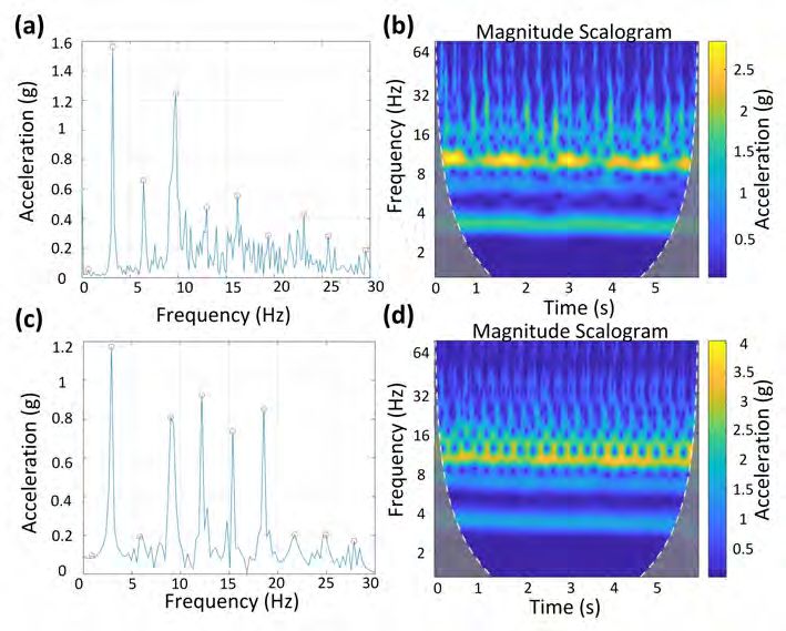
2       Hasti Hayati, David Eager, and Sebastian Oberst

that the spike in the anterior-posterior signals are approximately the stride-cuts
and were due to the hind-leg impacts [13]. The same results has been observed,
both through the time-domain and time-frequency domain analysis on racing
greyhounds [14, 9, 10]. Accelerometry has also been shown to be suited to study
indirectly different terrains or the effect of different terrains on the dynamics of
locomotion, a problem less often explored. Spence et al. used a custom designed
accelerometer backpack attached close the centre of mass (CoM) of a cockroach
to study the effect of leaf-litter as complex terrain on the locomotion dynamics
of rapid insects [11]. The peaks of the CoM dorsal-ventral acceleration on soft
surfaces were smaller compared to those belonging to running on rigid surfaces
[11].
    While incredibly robust and fast to compute, frequency domain approaches
do not provide the same level of information as time domain methods [15]. The
latter on the other hand, often fail to provide reliable measures or their ease of
application is significantly hampered either due to missing analysis frameworks
or due to the complexity of the analysis itself [16].
    In greyhound racing pushes the dogs to their physical limits which some-
times results in injuries and subsequent euthanization; to prevent this and to
develop countermeasures, the biomechanics and dynamics of greyhound gallop-
ing gait including the relationship to ground reaction forces need to be better
understood. This research uses an IMU to measure and then explain greyhound
characteristics galloping over two different terrains, wet sand and natural grass.
Using an IMU was chosen as it is capable of reliably recording field data for
a galloping greyhound. In addition to conducting a frequency domain analy-
sis, we also conducted a continuous wavelet transform (CWT) and an extended
time domain analysis based on the reconstructed phase space (RPS), making use
of nonlinear time series analysis, founded on nonlinear dynamics theory. While
more complex we hypothesise that the CWT and especially the RPS will provide
more information, beneficial to study the effect of different racing track grounds.

2     Methods
2.1   Experimental setup
Two oval-shaped greyhound race tracks of different surface type–wet sand and
natural grass–were selected.
    Six randomly selected greyhounds ran individually on a track with a grass
surface. The grass track was an oval-shaped with a turn radius of 84 m. Six ran-
domly selected greyhounds ran individually on a track with a wet sand surface.
The sand track was also oval-shaped with a turn radius of 53 m.
    Only galloping on the straight section of the tracks was analysed so as to
eliminate the effect of other possible variables such as Turning.
    To measure the dynamics, an in-house IMU device equipped with a 185 Hz
tri-axial accelerometer capable of measuring acceleration up to 16G was used.
The IMU allows tracking of tri-axial body rotation, tri-axial linear body acceler-
ation and tri-axial magnetic heading. Only the tri-axial linear accelerations were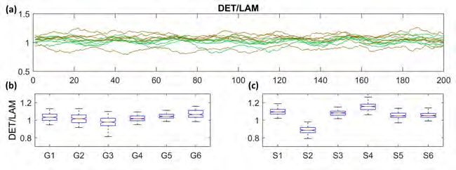
Recurrence plot quantification analysis of greyhound galloping gait     3

analysed in this study. A simultaneous kinematics study was performed using
two Sony DSC-RX10-III HFR cameras, one set to 50 fps to capture the entire
race, the other set to 500 fps to capture at least two full strides of the greyhound
with greater resolution. The HFR camera was mounted close to the finish line
ensuring greyhounds were at their highest speed and at a steady-state gallop.

Fig. 1. A greyhound galloping over a sand track with the IMU mounted approximately
above the greyhound’s centre of mass.

2.2   Frequency-domain, time-frequency domain analysis and phase
      space analysis
Fast Fourier Transform (FFT) is a powerful tool in signal processing which
applied in numerous fields [17]. The FFT is based on the discrete Fourier trans-
forms (DFT) but is much faster than DFT and allows to determine the dominant
modes (resonances) in a vibrating system. The DFT is defined as:
                             N
                             X −1
                    X(k) =          x(n)e−j2πn/k , k = 0, 1, ..., N             (1)
                             n=0

where x(n) is a finite data sequence in time-domain consists of N elements and
e−j2πn/k is a primitive N th root of 1 [18].

Continuous wavelet transform (CWT) is another strong tool in signal
processing which decomposes a time-series into time-frequency space. In other
words, using wavelets allows determining both the dominant modes and how
those modes vary with time. The CWT is a type of wavelet analysis that provides
an over-complete representation of a signal by letting the translation and scale
parameter of the wavelets vary continuously and is defined as:
                                −1
                             N           r     "           #
                             X
                                      0    δt ∗ (n − n0 δt
                    Wn (s) =       x(n )     Ψ                               (2)
                              0
                                           S 0       S
                               n =0

where S is the wavelet scale and Ψ is wavelet translation with ∗ symbolise a
complex conjunction [19].
   Although the use of FFTs and CWT, and linear-time-series analyses could
provide informative data with regards greyhound gait, they are limited and
4 Hasti Hayati, David Eager, and Sebastian Oberst
are not the best tools to understand complex and highly nonlinear dynamics
or transient processes of galloping greyhounds. Thus, frequency and wavelet
analysis are compared to each other and complemented by a recurrence plot
quantification analysis (RPQA) based on embedding the dynamics in the phase
space which is suitable to study nonlinear dynamics but also allows a study
of stochastic processes and non-stationary events [16]. These methods will be
briefly introduced.
Phase-space reconstruction (RPS) and recurrence plots (RP) Phase
space reconstruction is the foundation of nonlinear time series analysis that
allows the reconstruction of complete system dynamics using a single time se-
ries [20]. The most common approach for RPS time series is based on Takens’
delay embedding theorem [21]. Using this theorem, a single vector of the obser-
vations representing a chaotic system is used to reconstruct a multi-dimensional
system. The regenerated vectors can thus display numerous essential proper-
ties of its real time series provided that the embedding dimension is sufficiently
large [22].
RP is an advanced technique of nonlinear data analysis, introduced in late
1980’s [16]. It is a visualisation (or a graph) of a square matrix, in which the
matrix elements correspond to those times at which a state of a dynamical system
recurs (columns and rows correspond then to a time-delayed pair of values) [16,
23].
3 Results and discussion
FFT results The frequency domain results of a greyhound galloping on a
grass track and on a sand track are shown in Figure 2. There are three dominant
frequencies at 3.5 Hz, and 7 Hz and 10 Hz, cf. Figure 2(a,c). The 3.5 Hz frequency
is attributed to the gait frequency of the galloping greyhound (cycle) and 7 Hz
frequency is the step frequency. The 12 Hz frequency attributes to paw strikes
repeating four times each stride [14].
CWT results The discrete wavelet transform was applied on data indicated
as abrupt signal alterations shown is Figure 3(b,d), where the time-varying fre-
quency (Hz) is plotted against time (s). Magnitude (indicated by colour gradient)
refers to the value of the anterior-posterior acceleration. Abrupt changes in sig-
nals suggest anomaly in the gait, which may be caused by the design of the
track, such as the lack of a transition into and out of the bend and inconsistency
in the surface [14].
The CWT results of a greyhound galloping on a grass track and on a sand
track are shown in Figure 2(b,d).Recurrence plot quantification analysis of greyhound galloping gait 5
Fig. 2. (a) FFT plot of track with a grass surface. (b) CWT plot of track with a grass
surface. (c) FFT plot of track with a sand surface. (d) CWT plot of track with a sand
surface.
Three dominant frequency were observed around 3 Hz, 6 Hz and 10 Hz. The
high-power frequency is at approximate 10 Hz. The similar patterns are observed
in all data sets. Since the greyhounds are galloping straight they are in a pseudo
steady-state and no fluctuation in frequency and power is observed. However,
there are few high-power spots on the plots.
A higher power stride frequency is observed on grass compared to sand. The
CWT pattern on sand is more consistent which suggests a relative unchanging
surface condition. Fatigue during racing, indicated as abrupt signal alterations
has been observed from our recent work, where the CWT was applied on the
whole race rather than isolated straight running sections of the race [14].
3.1 Nonlinear time series method
RPS and RP results The averaged auto-mutual information (mi) determines
a suitable delay τ and applying then the global false nearest neighbour (fnn)
algorithm provides a suitable embedding dimension m to embed the time series
into a n-dimensional phase space. Both, τ and m are needed to span up the6 Hasti Hayati, David Eager, and Sebastian Oberst
phase space and to unfold the attracting set of the dynamics [24]. The phase
space is required to setup the RP matrices, to study the phase space diameter
and to a conduct recurrence plot quantification analysis [16]. The mi as a general
dependence (correlation) measure indicating how much of the information of the
previous sample is contained in subsequent sample points [25]. Table 1 lists the
identified delays τ and embedding dimensions m. As shown in [26], the delay
and the dimension alone can already provide hints on how the phase-space size
(pss) is calculated for the each RPS. From Table 1 it appears that the τ and m
for grass are slightly larger, indicating a tendency for higher dimensionality. A
higher sampling rate would facilitate the discrimination of different τ 1 .
Table 1. The delay τ , the embedding dimension m and the phase-space size (pss) are
given for accelerations of extracted track sections of grass (G) and sand (S).
Grass m τ pss Sand m τ pss
G1 4 5 14.5 S1 5 4 14.7
G2 4 4 16.8 S2 4 4 14.7
G3 5 5 16.0 S3 4 4 17.7
G4 4 4 14.8 S4 3 3 17.7
G5 4 4 15.5 S5 4 5 12.3
G6 4 4 18.6 S6 4 4 16.3
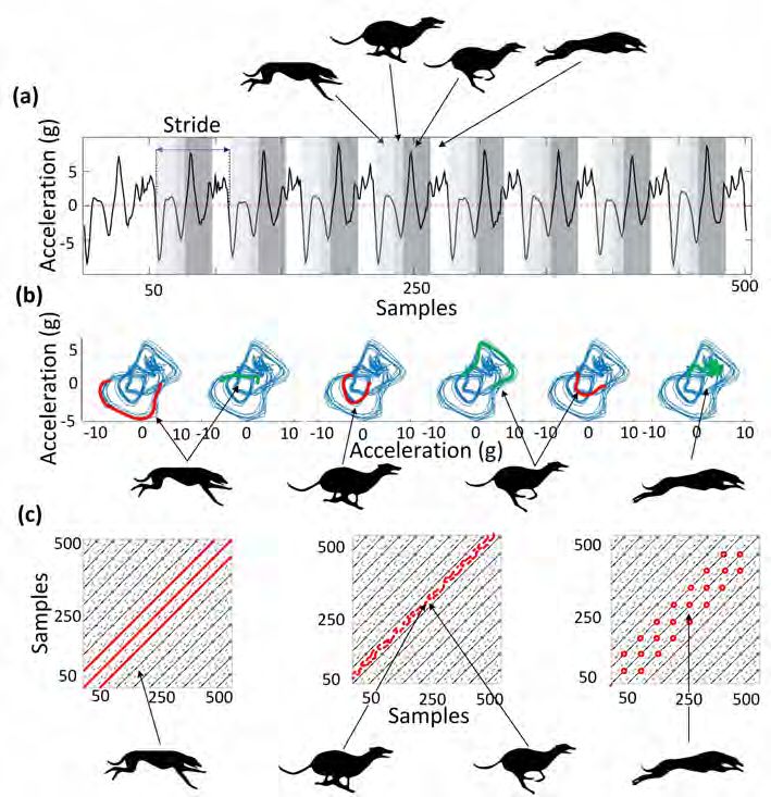
Figure 3 shows a sample of signal, represented in three different ways using
the time-domain (Figure 4.(a)), RPS (Figure 4.(b)), and RP (Figure 4.(c)). The
time-domain signals were synchronised with HFR videos in our recent work [14],
which is now used to correlate with RPS and RP representations. The phase
space indicates stable and unstable periodic orbits which are depicted in (c) as
solid and interrupted diagonal lines [27, 28].
1
The dimension estimate would not change.Recurrence plot quantification analysis of greyhound galloping gait 7 Fig. 3. (a) Time-domain signals (b), RPS plots, and (c) RP of a sample data set (greyhound galloping on a sand surface). Fig. 4. (a) RPS plots of grass surface. (b) RPs of grass surface. (c) RPS plots of sand surface. (d) RPs of sand surface.
8       Hasti Hayati, David Eager, and Sebastian Oberst

    Figure 4 shows the RPS and RP on sand and grass.On the RSP plots two
trajectories lying in the negative quadrant are due to foreleg strikes and the
compressed flight. The trajectories in the first quadrant are attributed to the
hind-leg strikes and the extended flight. The large trajectories in the third quad-
rant is attributed the fore-leg strikes and the second largest one is due to the
compressed flight. The large trajectory in the first quadrant is attributed to
the hind-leg strikes. The part with faster dynamics (high frequency content)
attributed to the extended flight its exact is, however, origin unknown.
    The following patterns is generally seen in all recurrence plots of all twelve
data-sets. A solid black diagonal represent a clear periodicity, the main running
cycle. The only clear periodicity in the current system is the main galloping
cycle of the greyhound at 3.5 Hz, indicated as solid black diagonal line, which is
also seen in the FFT and CWT plots. The two dashed-lines between each rigid
diagonal lines, are attributed to the compressed flight and hind-leg strikes, which
have about half the sampling points of the main cycle. The dot-shaped pattern
on the plots are also attributed to the extended flight (fast dynamics).
    The main observation based on Figure 4 is that the RPS of sand surface
appear clearer than that of grass. Sand surfaces are better maintained than grass
surfaces in general resulting in a smoother arena ground and more consistent
gallop. The large trajectories in the third quadrant, which are attributed to the
fore-leg strikes, appear relatively larger on sand than on grass, which may suggest
a harder surface. It has been observed in our recent work that sand surface is
harder than the grass one but was not seen in the time-domain and frequency
domain analysis of the signal [14]. However, using RPS representations, shows
the potential to derive a method to estimate the difference in the surface stiffness
relatively compared with each other.
    It can be seen from Figure 4 that the black rigid lines, attributed to stride
frequency, are clear on both sand and grass surface. The extended flight dynamic
is more distinguishable in RP representation than the RPS, where it was rep-
resented as more random appearing trajectories. The RP representation could
reveal dynamics which could not be observed in other signal representations, i.e.
extended flight dynamics which is seems to be represented as a positive random
trajectories on RPS plots. However, the low frequency range does not allow to
see more details. Also the correlation with other measurements (eg rotational
sensors, videos) has not been conducted specifically for the purpose of studying
these fast dynamics during extended flight, which is an outstanding task for the
near future.

Cross recurrence quantification analysis (CRQA) Figure 5 shows the
CRQA results of all samples via three different measurements of determinism
(DET), divided by its laminarity (LAM); DET and LAM are calculated as per-
centage of recurrence points which form diagonal and vertical lines [16]. DET
expresses how deterministic, i.e. predictable the data is as opposed to random
data. For fully deterministic data, such as for a sinusoidal or a quasi-periodic
signal, a value of one is obtained; for deterministic chaos, a value between 1 and
Recurrence plot quantification analysis of greyhound galloping gait 9
0 and for random data a value of of 0 is expected. LAM indicates whether a
system remains in a certain state or not. In both plots, the green lines attribute
to the grass surface while the brown lines represent the sand surface. As can be
observed from Figure 5, the ratio of DET to LAM approximates unity which is
indicative for having similarly high values. Both individual metrics where oscil-
lating in phase at around at a value of around 0.8, which shows that the system
is not fully predictable and that changes of states influence proportionally pre-
dictability. From Figure 3 one can see that the main period, shown up at diagonal
line (and related to the main frequency of the system) is predictable but that
the subsequent motions, are more recurrent than strictly periodic.
To test whether the measurements are significantly different, notched box
plots are used. The notches indicate 95% confidence intervals (CI); non-overlapping
confidence intervals indicate statistically significant results. The data related to
sand is has slightly higher values; S2 seems to be a very different measure-
ment though and could be treated as outlier. Comparing the CI between the
two groups (removing in both cases the boxplot with the minimum and the
maximum median) indicates that the ratio DET/LAM for the sand tracks is
significantly different to those of grass (average CI for grass is [1.033, 1.018]
while that of sand is [1.09, 1.08]. Taking the median values of all DET/LAM
for each of the two types of tracks and using a 1-way ANOVA test (assuming a
parametric distribution) provides non-significant results (df = 13, SS = 0.05002,
F = 0.97, p = 0.3434); removing the outliers, however, provides significant differ-
ences between sand and grass at the 5% significance level (df = 7, SS = 0.01531,
F = 6.11, p = 0.0484).
Fig. 5. (a) determinism/laminarity of a greyhound galloping an grass (represented by
green lines) and sand (represented by brown lines). (b) The notched box plots of grass.
(c) The notched box plots of sand.
4 Conclusion
In this work the nonlinear-time-series-analysis techniques of RPS and RP were
applied for the first time to study greyhound dynamics. IMU signals measured10 Hasti Hayati, David Eager, and Sebastian Oberst
from greyhounds galloping on grass and surfaces were used to investigate whether
these methods can detect a difference in the mechanical properties of the rac-
ing track surface. The results showed that using RPS and RP, the mechanical
properties of the track surface can be generally be compared with each other.
For the first time, the galloping gait segments of greyhounds were correlated
with the RPS and RP representations. The overall motion can be classified as
having a period-4 limit cycle, whereas only the main cycle is clearly periodic.
RPS plots could identify the harder surface type; RP could identify dynamics on
the system which were difficult to detect using other methods. Similar to iden-
tifying instabilities in technical systems long time before they occur [29]), RP
and RPQA may be used extract otherwise hidden information to identify motion
components from the attractor’s trajectory as potential source of injuries. Using
RPQA measures we showed that the ratio of determinism and laminarity shows
significantly different results between grass and sand. Using a Bonferroni cor-
rection would explicitly allow to study the group differences. While the different
parts of the gait cycle have been distinguished a closer look at the recurrence
plots and their quantification analysis may reveal differences in step pattern.
The high-frequency content in the flight phase has not yet been fully analysed,
for which potentially a higher sampling rate would be required.
References
1. E. Barrey and P. Galloux, “Analysis of the equine jumping technique by accelerom-
etry,” Equine Veterinary Journal, vol. 29, no. S23, pp. 45–49, 1997.
2. A. Muro-De-La-Herran, B. Garcia-Zapirain, and A. Mendez-Zorrilla, “Gait analysis
methods: An overview of wearable and non-wearable systems, highlighting clinical
applications,” Sensors, vol. 14, no. 2, pp. 3362–3394, 2014.
3. T. Witte, K. Knill, and A. Wilson, “Determination of peak vertical ground reaction
force from duty factor in the horse (equus caballus),” Journal of Experimental
Biology, vol. 207, no. 21, pp. 3639–3648, 2004.
4. H. Chateau, L. Holden, D. Robin, S. Falala, P. Pourcelot, P. Estoup, J. Denoix, and
N. Crevier-Denoix, “Biomechanical analysis of hoof landing and stride parameters
in harness trotter horses running on different tracks of a sand beach (wet to dry)
and on an asphalt road,” Equine Veterinary Journal, vol. 42, pp. 488–495, 2010.
5. S. D. Starke, T. H. Witte, S. A. May, and T. Pfau, “Accuracy and precision of
hind limb foot contact timings of horses determined using a pelvis-mounted inertial
measurement unit,” Journal of biomechanics, vol. 45, no. 8, pp. 1522–1528, 2012.
6. S. Viry, R. Sleimen-Malkoun, J.-J. Temprado, J.-P. Frances, E. Berton, M. Lau-
rent, and C. Nicol, “Patterns of horse-rider coordination during endurance race: a
dynamical system approach,” PloS one, vol. 8, no. 8, p. e71804, 2013.
7. A.-M. Pendrill and D. Eager, “Velocity, acceleration, jerk, snap and vibration:
forces in our bodies during a roller coaster ride,” Physics Education, vol. 55, no. 6,
p. 065012, 2020.
8. N. F. Ribeiro and C. P. Santos, “Inertial measurement units: A brief state of the
art on gait analysis,” in 2017 IEEE 5th Portuguese Meeting on Bioengineering
(ENBENG), pp. 1–4, IEEE, 2017.Recurrence plot quantification analysis of greyhound galloping gait 11
9. H. Hayati, D. Eager, and T. Brown, “A study of rapid tetrapod running and turning
dynamics utilizing inertial measurement units in greyhound sprinting,” American
Society of Mechanical Engineers, 2017.
10. H. Hayati, P. Walker, F. Mahdavi, R. Stephenson, T. Brown, and D. Eager, “A
comparative study of rapid quadrupedal sprinting and turning dynamics on dif-
ferent terrains and conditions: racing greyhounds galloping dynamics,” American
Society of Mechanical Engineers, 2018.
11. A. J. Spence, S. Revzen, J. Seipel, C. Mullens, and R. J. Full, “Insects running on
elastic surfaces,” Experimental Biology, vol. 213, no. 11, pp. 1907–1920, 2010.
12. D. Eager, A.-M. Pendrill, and N. Reistad, “Beyond velocity and acceleration: Jerk,
snap and higher derivatives,” European J. of Physics, vol. 37, no. 6, pp. 65–68, 2016.
13. A. M. Wilson, J. Lowe, K. Roskilly, P. E. Hudson, K. Golabek, and J. McNutt,
“Locomotion dynamics of hunting in wild cheetahs,” Nature, vol. 498, no. 7453,
pp. 185–189, 2013.
14. H. Hayati, F. Mahdavi, and D. Eager, “Analysis of agile canine gait characteristics
using accelerometry,” Sensors, vol. 19, no. 20, 2019.
15. J. P. Zbilut and N. Marwan, “The wiener–khinchin theorem and recurrence quan-
tification,” Physics Letters A, vol. 372, no. 44, pp. 6622–6626, 2008.
16. N. Marwan, M. C. Romano, M. Thiel, and J. Kurths, “Recurrence plots for the
analysis of complex systems,” Physics reports, vol. 438, no. 5-6, pp. 237–329, 2007.
17. J. W. Cooley, P. A. Lewis, and P. D. Welch, “The fast fourier transform and its
applications,” IEEE Transactions on Education, vol. 12, no. 1, pp. 27–34, 1969.
18. M. H. Hayes, Statistical digital signal processing. John Wiley & Sons, 2009.
19. C. Torrence and G. P. Compo, “A practical guide to wavelet analysis,” Bulletin of
the American Meteorological society, vol. 79, no. 1, pp. 61–78, 1998.
20. E. Bradley and H. Kantz, “Nonlinear time-series analysis revisited,” Chaos: An
Interdisciplinary Journal of Nonlinear Science, vol. 25, no. 9, p. 097610, 2015.
21. F. Takens, “Detecting strange attractors in turbulence,” in Dynamical systems and
turbulence, Warwick 1980, pp. 366–381, Springer, 1981.
22. C. Frazier and K. M. Kockelman, “Chaos theory and transportation systems,”
Transportation Research Record, vol. 1897, no. 1, pp. 9–17, 2004.
23. B. Goswami, “A brief introduction to nonlinear time series analysis and recurrence
plots,” Vibration, vol. 2, pp. 332–368, 2020.
24. H. Kantz and T. Schreiber, Nonlinear time series analysis, vol. 7. Cambridge
University Press, 2004.
25. S. Oberst, J. Lai, and T. Evans, “Key physical wood properties in termite foraging
decisions,” The Royal Society Interface, vol. 15, no. 149, p. 20180505, 2018.
26. S. Oberst, J. Baetz, G. Campbell, F. Lampe, J. C. Lai, N. Hoffmann, and M. Mor-
lock, “Vibro-acoustic and nonlinear analysis of cadavric femoral bone impaction
in cavity preparations,” International Journal of Mechanical Sciences, vol. 144,
pp. 739–745, 2018.
27. S. Oberst, S. Marburg, and N. Hoffmann, “Determining periodic orbits via nonlin-
ear filtering and recurrence spectra in the presence of noise,” Procedia Engineering,
vol. 199, pp. 772–777, 2017.
28. S. Oberst, R. K. Niven, D. Lester, A. Ord, B. Hobbs, and N. Hoffmann, “De-
tection of unstable periodic orbits in mineralising geological systems,” Chaos: An
Interdisciplinary Journal of Nonlinear Science, vol. 28, no. 8, p. 085711, 2018.
29. M. Stender, S. Oberst, M. Tiedemann, and N. Hoffmann, “Complex machine dy-
namics: systematical recurrence analysis of disk brake vibration data,” Nonlinear
Dynamics, vol. 97, no. 4, pp. 2483–2497, 2019.You can also read