Reduced-order Model for Fluid Flows via Neural Ordinary Differential Equations
←
→
Page content transcription
If your browser does not render page correctly, please read the page content below
Reduced-order Model for Fluid Flows via Neural Ordinary Differential Equations
                                                                             Carlos J.G. Rojas 1 , Andreas Dengel 1 , Mateus Dias Ribeiro 1
                                                                                       1
                                                                                      German Research Center for Artificial Intelligence - DFKI
                                                                        carlos.gonzalez rojas@dfki.de, andreas.dengel@dfki.de, mateus.dias ribeiro@dfki.de
arXiv:2102.02248v1 [physics.flu-dyn] 3 Feb 2021

                                                                              Abstract                                the physical behaviour for unseen parameters and that can
                                                                                                                      extrapolate forward in time using the minimal amount of full
                                                    Reduced order models play an important role in the design,        order simulations (Benner, Gugercin, and Willcox 2015).
                                                    optimization and control of dynamical systems. In recent
                                                    years, there has been an increasing interest in the applica-         The projection-based reduced order modeling is one of
                                                    tion of data-driven techniques for model reduction that can       the most popular approaches to construct surrogate models
                                                    decrease the computational burden of numerical solutions,         of dynamical systems. This framework reduces the degrees
                                                    while preserving the most important features of complex           of freedom of the numerical simulations using a transfor-
                                                    physical problems. In this paper, we use the proper orthogo-      mation into a suitable low-dimensional subspace. Then, the
                                                    nal decomposition to reduce the dimensionality of the model       state variable in the governing equations is rewritten in terms
                                                    and introduce a novel generative neural ODE (NODE) archi-         of the reduced subspace and finally the PDE equations are
                                                    tecture to forecast the behavior of the temporal coefficients.
                                                                                                                      converted into a system of ODEs that can be solved using
                                                    With this methodology, we replace the classical Galerkin pro-
                                                    jection with an architecture characterized by the use of a con-   classical numerical techniques (Benner, Gugercin, and Will-
                                                    tinuous latent space. We exemplify the methodology on the         cox 2015). In the field of fluid mechanics, the Proper Or-
                                                    dynamics of the Von Karman vortex street of the flow past a       thogonal Decomposition (POD) method is widely applied in
                                                    cylinder generated by a Large-eddy Simulation (LES)-based         the dimensionality reduction of the FOM and the Galerkin
                                                    code. We compare the NODE methodology with an LSTM                method is used for the projection onto the governing equa-
                                                    baseline to assess the extrapolation capabilities of the gener-   tions. These methodologies are preferred because an orthog-
                                                    ative model and present some qualitative evaluations of the       onal normal basis simplifies the complexity of the projected
                                                    flow reconstructions.                                             mathematical operators and the truncated basis of the POD
                                                                                                                      is optimal in the least squares sense, retaining the dominant
                                                                          Introduction                                behaviour through the most energetic modes. The projection
                                                                                                                      on the governing equations maintain the physical structure
                                                  Modeling and simulation of dynamical systems are essential          of the model, but the truncation of the modes can affect the
                                                  tools in the study of complex phenomena with applications           accuracy of the results in nonlinear systems and it may also
                                                  in chemistry, biology, physics and engineering, among other         be restricted to stationary and time periodic problems. Fur-
                                                  relevant fields. These tools are particularly useful in the con-    thermore, the projection is intrusive, requiring different set-
                                                  trol and design of parametrized systems in which the depen-         tings for each problem, and it is limited to explicit and closed
                                                  dence on properties, initial conditions and other configura-        definitions of the mathematical models (San, Maulik, and
                                                  tions requires multiple evaluations of the system response.         Ahmed 2019). Some of these problems have been addressed
                                                  However, there are some limitations when performing nu-             with the search of closure models that compensates the in-
                                                  merical simulations of systems where nonlinearities, and a          formation losses produced by the truncated modes (Mou
                                                  wide range of spatial and time scales leads to unmanageable         et al. 2020; Mohebujjaman, Rebholz, and Iliescu 2019; San
                                                  demands on computational resources. The latter is the case          and Maulik 2018b,a) and with the construction of a data
                                                  of engineering fluid flow problems where the range of scales        driven reduced ”basis” that also provides optimality after
                                                  involved increase with the value of the Reynolds number and         the time evolution (Murata, Fukami, and Fukagata 2020; Liu
                                                  the cost of simulating a full-order model (FOM) using tech-         et al. 2019; Wang et al. 2016).
                                                  niques such as DNS or LES is very high. One of the possi-
                                                                                                                         We present an alternative methodology to evolve the dy-
                                                  ble solutions to reduce the expensive computational cost is
                                                                                                                      namics of the system in the reduced space using a data-
                                                  to introduce an alternative, cheaper and faster representation
                                                                                                                      driven approach. We use the POD to compute the modes and
                                                  that retains the characteristics provided by the FOM without
                                                                                                                      the temporal coefficients of a fluid flow simulation and then
                                                  sacrificing the accuracy of the general physical behaviour.
                                                                                                                      we apply a non-supervised autoencoder approach to learn
                                                  The idea is to construct a methodology able to generalize
                                                                                                                      the dynamics of a latent space. The addition of a neural ODE
                                                  Copyright © 2021, Association for the Advancement of Artificial     (Chen et al. 2019; Rubanova, Chen, and Duvenaud 2019)
                                                  Intelligence (www.aaai.org). All rights reserved.                   block in the middle of the autoencoder model provides a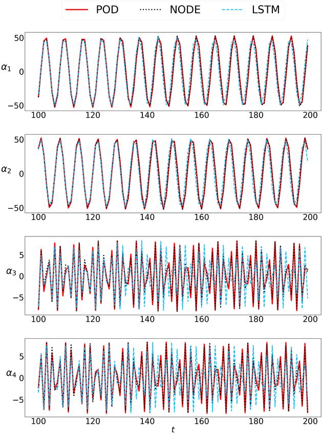
Figure 1: POD-NeuralODE ROM methodology.

continuous learning block that is encoded using a feed for-            LES Model For The Flow Past a Cylinder
ward neural network and that can be solved numerically to           The dynamics of the Von Karman vortex street of the flow
determine the future states of the input variables. Several         past a cylinder were solved by the LES filtered governing
works have proposed machine learning models to replace              equations for the balance of mass (1), and momentum (2),
the Galerkin projection step or to improve their capabilities,      which can be written as follows:
and different architectures such as feedforward or recurrent
networks has been applied with demonstrated good perfor-                                    ∂ ρ̄ ∂(ρ̄ũi )
mance in academic and practical fluid flow problems (Pawar                                      +          =0                         (1)
                                                                                            ∂t    ∂xi
et al. 2019; Imtiaz and Akhtar 2020; Eivazi et al. 2020; Lui
and Wolf 2019; Portwood et al. 2019; Maulik et al. 2020a,b).
The main advantage of the neural ODE generative model is                ∂(ρ̄ũi ) ∂(ρ̄ũi u˜j )     ∂            ∂ u˜j      ∂ ũi
                                                                                 +              =         ρ̄ν̄          +
that the learning is posed as a non-supervised task using a               ∂t        ∂xj            ∂xj           ∂xi        ∂xj
continuous representation of the physical behavior. In our                                                                           (2)
                                                                                   2 ∂ u˜k                             ∂ p̄
view, the neural ODE block can be interpreted as an im-                          − ρ̄ν̄        δij − ρ̄τij sgs −            + ρ̄gi
plicit differential operator that is not restricted to a specific                  3 ∂xk                             ∂xi
differential equation. This setting provides more flexibility          In the previous equations, u represents the velocity, ρ is
than the projection over the governing equations because it         the fluid density, and ν is the dynamic viscosity. These equa-
addresses the learning problem with an operator that is in-         tions are solved numerically using the PIMPLE algorithm
formed and corrected by the training data.                          (Weller et al. 1998), which is a combination of PISO (Pres-
                                                                    sure Implicit with Splitting of Operator) by Issa (1986) and
                       Methodology                                  SIMPLE (Semi-Implicit Method for Pressure-Linked Equa-
In this work we use a Large-eddy Simulation (LES) model             tions) by Patankar (1980). This approach obtains the tran-
to approximate the behavior of the fluid flow dynamical sys-        sient solution of the coupled velocity and pressure fields by
tem. As it is the case in many fluid flow problems, the dis-        applying the SIMPLE (steady-state) procedure for every sin-
crete solution has a spatial dimension larger than the size of      gle time step. Once converged, a numerical time integration
the temporal domain. For this reason, we apply the snapshot         scheme (e.g. backward) and the PISO procedure are used to
POD to construct the reduced order model in order to have           advance in time until the simulation is complete. Further-
a tractable computation. The POD finds a new basis repre-           more, the unresolved subgrid stresses, τij sgs , are modeled
sentation that maximizes the variance in the data, and has          in terms of the subgrid-scale eddy viscosity νT using the dy-
the minimum error of the reconstructions in a least squares         namic k-equation approach by Kim and Menon (1995).
sense. In addition, the dimensionality reduction is easily per-        The setup of the problem is described as follows. The
formed because the components of the new basis are ordered          computational domain comprehends a 2D channel with
by their contribution to the recovery of the data.                  760 mm in the stream-wise direction and 260 mm in the di-
   The main block in the Neural ODE-ROM methodology                 rection perpendicular to the flow. The cylinder is located be-
is concerned with the forecast of the temporal coefficients         tween the upper and bottom walls of the channel at 115 mm
provided by the snapshot POD. Here we apply a genera-               away from the inlet (left wall). A constant radial velocity
tive neural ODE model that takes the temporal coefficients,         of 0.6 m/s with random radial/vertical fluctuations in com-
learns their dynamical evolution and provides an adequate           bination with a zero-gradient outflow condition and non-
model to extrapolate at the desired time steps. Finally, we         slip walls on the top/bottom/cylinder walls are imposed as
can forecast the evolution of the temporal coefficients and         boundary conditions. Furthermore, a laminar dynamic vis-
reconstruct the behavior of the flow with the spatio-temporal       cosity of 1 × 10⁻⁴ m2 /s and a cylinder diameter of 40 mm
expansion used in the POD.                                          further characterizes the flow with a Reynolds number of
   The general methodology is represented in the Fig. 1 and         240 (Re = 0.6 × 0.04/1 × 10−4 = 240). The Central differ-
more details about each of the building blocks is presented         encing scheme (CDS) was used for the discretization of both
in the following sections.                                          convective and diffusive terms of the momentum equation,
as well as an implicit backward scheme for time integration. where each row contains a flattened array with the fluctu-
A snapshot of the velocity components in both radial and ating components of the velocity in the x and y directions
axial directions at time = 100 is shown in the Fig. 2. for a given time step. If the discretization used for the
FOM simulation has dimensions Nx , Ny and Nt , then the
flattened representation is a vector with length 2 · Nx · Ny
and the matrix Y has dimensions Nt × (2 · Nx · Ny ).
• Build the correlation matrix K and compute its eigenvec-
tors aj :
K = Y Y >, (4)
Kaj = λj aj . (5)
Alternatively, one can directly compute the eigenvalues
and eigenvectors using the singular value decomposition
(SVD) of the snapshot matrix.
• Choose the reduced dimension of the model: As described
Figure 2: Snapshot of the flow field at t = 100. in the literature, larger eigenvalues are directly related
with the dominant characteristics of the dynamical sys-
Proper Orthogonal Decomposition tem while small eigenvalues are associated with perturba-
The proper orthogonal decomposition (POD) is known un- tions of the dynamic behavior. The criterion to select the
der a variety of names such as Karhunen-Loeve expan- components for the new basis is to maximize the relative
sion, Hotelling transform and principal component analysis information content I(N ) using the minimal amount of
(Liang et al. 2002). This tool was developed in the field of components N necessary to achieve a desired percentage
probability theory to discover interdependencies within vec- of recovery (Schilders et al. 2008).
tor data and introduced in the fluid mechanics community PN
by Berkooz, Holmes, and Lumley (1993). Once the interde- i=1 λi
pendencies in the data are discovered, it is possible to reduce I(N ) = PN t
(6)
its dimensionality. i=1 λi
The formulation of the dimensionality reduction starts • Finally, we compute the spatial modes using the tempo-
with some samples of observations provided by experimen- ral coefficients in the reduced dimensional space and the
tal results or obtained through the numerical solution of a Ansatz decomposition of the POD:
full order model that characterizes the physical problem.
These samples are rearranged in an ensemble matrix of snap- N
X
shots Y where each row has the state of the dynamical sys- u0 = αi (t)ψi (x), (7)
tem at a given time step. Then, the correlation matrix of the i=1
elements in Y is computed and their eigenvectors are used
as an orthogonal optimal new basis for the reduced space. N
1 X
In the following list we summarize the main steps used ψi (x) = αi (tj )u0 (tj ). (8)
λi j=1
for the construction of the snapshot POD:
• Take snapshots : simulate the dynamical system and sam-
ple its state as it evolves. Neural Ordinary Differential Equations
• Compute the fluctuating components of the velocity using The neural ordinary differential methodology (Chen et al.
the Reynolds decomposition of the flow: 2019) can be interpreted as a continuous counterpart of tradi-
tional models such as recurrent or residual neural networks.
In order to formulate this model, the authors drew a parallel
u = u + u0 , (3)
between the classical composition of a sequence in terms of
where u is the temporal mean of the solutions given by previous states and the discretization methods used to solve
the FOM model. differential equations:
• Assemble the matrix Y with the snapshots in the follow-
ing form: ht+1 = ht + f (ht , θ). (9)
0
ux (x1 , y1 , t1 ) ... u0y (xNx , yNy , t1 )
0 0
In the limit case of sufficient small steps (equivalent to
ux (x1 , y1 , t2 ) ... uy (xNx , yNy , t2 ) an increase of the layers) is possible to write a continuous
. . .
Y =
parametrization of the hidden state derivative:
. . .
. . . dh(t)
u0x (x1 , y1 , tNt ) ... u0y (xNx , yNy , tNt ) = f (ht , θ), (10)
dt
Model Hyperparameter Range Best
latent dimension 3-6 6
ht = ODESolver(h0 , f (ht , θ)). (11) layers encoder 1-5 4
units encoder 10-50 10
The function f defining the parametrization of the deriva- Neural ODE units node 10-50 12
tive can be approximated using a neural network and the val- layers decoder 1-5 4
ues of hidden states ht at different time steps are computed units decoder 10-50 41
using numerical ODE solvers (Chen et al. 2019). learning rate 0.001 - 0.1 0.0015
We apply the neural ODE time-series generative approach layers 10-60 49
presented in the Fig. 3 to model the evolution of the tem- LSTM units 1-5 1
poral modes provided by the proper orthogonal decomposi- learning rate 0.001 - 0.1 0.0081
tion. This approach can be interpreted as a variational au-
toencoder architecture with an additional neural ODE block Table 1: Hyperparameters used in the models.
after the sampling of the codings. This block maps the vector
of the initial latent state zt0 to a sequence of latent trajecto-
ries using the ODE numerical solver while a neural network
f (ht , θ) learns the latent dynamics necessary to have a good
reconstruction of the input data.
After the training process, the latent trajectories are easily
extrapolated with the redefinition of the temporal bounds in
the ODE solver. Some of the advantages of this strategy are
that it does not need an explicit formulation of the physical
laws to forecast the temporal modes, and in consequence, the
method does not resort onto projection methodologies. Fur-
thermore, the parametrization using a neural network gives
an accurate nonlinear approximation of the derivative with-
out a predefined mathematical structure.
Results
In this section, we evaluate the performance of the genera-
tive neural ODE model in the forecasting of the temporal co-
efficients. For this assessment, we apply the proper orthogo-
nal decomposition over 300 snapshots of simulated data ob-
tained with the LES code and take the first 8 POD modes
achieving a 99 % of recovery according to the relative in-
formation content. For the deployment of the neural ODE
model (NODE) we take the first 75 time steps for the train-
ing set, the following 25 time steps for the validation of the
model and the last 200 time steps for the test set. Further-
more, we employ as a baseline model an LSTM sequence to
vector architecture as proposed in Maulik et al. with a win-
dow size of 10 time steps and a batch size of 15 sequences.
We tuned the hyperparameters necessary for both models
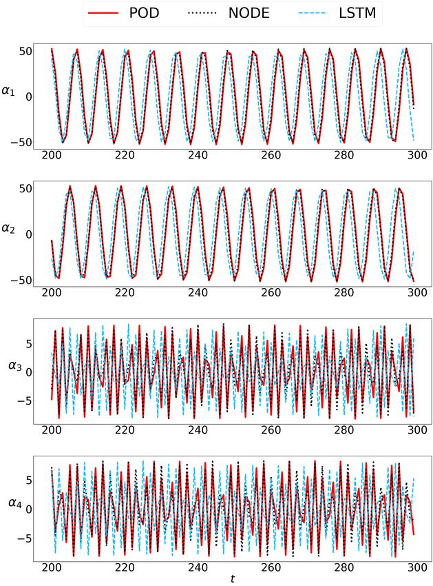
adopting a random search and chose the best configuration Figure 5: Reconstruction of POD temporal coefficients using
given the performance on the validation set. The evolution NODE vs LSTM , t ∈ [100, 200].
of the loss for the best model is shown in Fig. 4 and the set
of hyperparameters employed are presented in Table 1. The time-series prediction for the first four temporal co-
efficients in the test set is shown in Fig. 5. This plot presents
the ground truth values of the POD time coefficients, the
baseline produced using an LSTM architecture and the pre-
dictions by the proposed generative NODE model for the
first 100 time steps in the test window. We notice that the
baseline and the NODE model learned adequately the evo-
lution of the two most dominant coefficients, but the per-
formance of the NODE model is significantly better for the
third and four time coefficients. Additionally, the quality of
Figure 4: Loss Generative NODE model. the prediction using the LSTM model for the last 100 time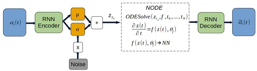
Figure 3: Generative VAE with Neural ODE.

steps in the test set deteriorates with the evolution of the time   figure shows with more details how the physical response of
steps even for α1 and α2 as seen in Fig. 6 . One of the pos-        the reduced order model gives a satisfactory approximation
sible reasons for this is that the autoregressive nature of the     of the flow behavior.
predictions in the LSTM model is prone to the accumulation
of errors as Maulik et al. pointed out in their study (Maulik
et al. 2020b).

                                                                    Figure 7: Contours of fluctuating component u0x , t = 300.

Figure 6: Reconstruction of POD temporal coefficients using
NODE vs LSTM, t ∈ [200, 300].

   After the training and validation process, we reconstruct
                                                                          Figure 8: Probe positioned behind the cylinder.
the velocity fluctuating component u0x using the Ansatz of
the proper orthogonal decomposition with the temporal co-
efficients forecasted for the test set. Observing the Fig. 7           The data and code that support this study is provided at
is possible to notice that the contour generated with the re-       https://github.com/CarlosJose126/NeuralODE-ROM.
duced order model provides an adequate recovery of the flow
features with only slight differences in some vortexes. In                               Conclusions
addition, we also present the fluctuation time history for a        We presented a methodology to produce reduced order mod-
probe located downstream from the cylinder in Fig. 8. This          els using a neural ODE generative architecture for the evo-
lution of the temporal coefficients. The neural ODE model Maulik, R.; Mohan, A.; Lusch, B.; Madireddy, S.; Bal-
was able to learn appropriately the hidden dynamics of the aprakash, P.; and Livescu, D. 2020b. Time-series learning
temporal coefficients without having the propagation of er- of latent-space dynamics for reduced-order model closure.
rors common in the autoregressive architectures. Another Physica D: Nonlinear Phenomena 405: 132368.
advantage of this methodology is that the learning is posed Mohebujjaman, M.; Rebholz, L.; and Iliescu, T. 2019. Phys-
as an unsupervised task without the requirement to divide ically constrained data-driven correction for reduced-order
the whole sequence in smaller training windows with labels. modeling of fluid flows. International Journal for Numeri-
We also remark that the continuous nature of the neural ODE cal Methods in Fluids 89(3): 103–122.
block is crucial for the good extrapolation capabilities of the
methodology. Finally, we expect to test the capabilities of Mou, C.; Liu, H.; Wells, D. R.; and Iliescu, T. 2020.
this methodology with other physical problems and also to Data-driven correction reduced order models for the quasi-
extend the method for parametric dynamical systems. geostrophic equations: a numerical investigation. Inter-
national Journal of Computational Fluid Dynamics 34(2):
147–159.
References
Murata, T.; Fukami, K.; and Fukagata, K. 2020. Nonlinear
Benner, P.; Gugercin, S.; and Willcox, K. 2015. A Survey of
mode decomposition with convolutional neural networks for
Projection-Based Model Reduction Methods for Parametric
fluid dynamics. Journal of Fluid Mechanics 882: A13.
Dynamical Systems. SIAM Review 57(4): 483–531.
Patankar, S. V. 1980. Numerical heat transfer and fluid flow.
Berkooz, G.; Holmes, P.; and Lumley, J. L. 1993. The Washington: Hemisphere Publishing Corporation.
Proper Orthogonal Decomposition in the Analysis of Turbu-
lent Flows. Annual Review of Fluid Mechanics 25(1): 539– Pawar, S.; Rahman, S. M.; Vaddireddy, H.; San, O.;
575. Rasheed, A.; and Vedula, P. 2019. A deep learning en-
abler for nonintrusive reduced order modeling of fluid flows.
Chen, R. T. Q.; Rubanova, Y.; Bettencourt, J.; and Duve- Physics of Fluids 31(8): 085101.
naud, D. 2019. Neural Ordinary Differential Equations.
arXiv:1806.07366 [cs, stat] ArXiv: 1806.07366. Portwood, G. D.; Mitra, P. P.; Ribeiro, M. D.; Nguyen, T. M.;
Nadiga, B. T.; Saenz, J. A.; Chertkov, M.; Garg, A.; Anand-
Eivazi, H.; Veisi, H.; Naderi, M. H.; and Esfahanian, V. kumar, A.; Dengel, A.; et al. 2019. Turbulence forecasting
2020. Deep neural networks for nonlinear model order re- via Neural ODE. arXiv preprint arXiv:1911.05180 .
duction of unsteady flows. Physics of Fluids 32(10): 105104.
Rubanova, Y.; Chen, R. T.; and Duvenaud, D. 2019. Latent
Imtiaz, H.; and Akhtar, I. 2020. POD-based Reduced-Order ODEs for Irregularly-Sampled Time Series. arXiv preprint
Modeling in Fluid Flows using System Identification Strat- arXiv:1907.03907 .
egy. In 2020 17th International Bhurban Conference on Ap- San, O.; and Maulik, R. 2018a. Machine learning closures
plied Sciences and Technology (IBCAST), 507–512. Islam- for model order reduction of thermal fluids. Applied Mathe-
abad, Pakistan: IEEE. matical Modelling 60: 681–710.
Issa, R. 1986. Solution of the implicitly discretised fluid flow San, O.; and Maulik, R. 2018b. Neural network closures
equations by operator-splitting. Journal of Computational for nonlinear model order reduction. Advances in Computa-
Physics 62(1): 40 – 65. tional Mathematics 44(6): 1717–1750.
Kim, W.-W.; and Menon, S. 1995. A new dynamic one- San, O.; Maulik, R.; and Ahmed, M. 2019. An artificial
equation subgrid-scale model for large eddy simulations. neural network framework for reduced order modeling of
Liang, Y.; Lee, H.; Lim, S.; Lin, W.; Lee, K.; and Wu, transient flows. Communications in Nonlinear Science and
C. 2002. PROPER ORTHOGONAL DECOMPOSITION Numerical Simulation 77: 271–287.
AND ITS APPLICATIONS—PART I: THEORY. Jour- Schilders, W. H. A.; van der Vorst, H. A.; Rommes, J.; Bock,
nal of Sound and Vibration 252(3): 527–544. ISSN H.-G.; de Hoog, F.; Friedman, A.; Gupta, A.; Neunzert, H.;
0022460X. doi:10.1006/jsvi.2001.4041. URL https:// Pulleyblank, W. R.; Rusten, T.; Santosa, F.; Tornberg, A.-
linkinghub.elsevier.com/retrieve/pii/S0022460X01940416. K.; Bonilla, L. L.; Mattheij, R.; and Scherzer, O., eds. 2008.
Liu, Y.; Wang, Y.; Deng, L.; Wang, F.; Liu, F.; Lu, Y.; and Model Order Reduction: Theory, Research Aspects and Ap-
Li, S. 2019. A novel in situ compression method for CFD plications, volume 13 of Mathematics in Industry. Berlin,
data based on generative adversarial network. Journal of Heidelberg: Springer Berlin Heidelberg.
Visualization 22(1): 95–108. Wang, M.; Li, H.-X.; Chen, X.; and Chen, Y. 2016. Deep
Lui, H. F. S.; and Wolf, W. R. 2019. Construction of Learning-Based Model Reduction for Distributed Parameter
reduced-order models for fluid flows using deep feedforward Systems. IEEE Transactions on Systems, Man, and Cyber-
neural networks. Journal of Fluid Mechanics 872: 963–994. netics: Systems 46(12): 1664–1674.
Weller, H. G.; Tabor, G.; Jasak, H.; and Fureby, C. 1998.
Maulik, R.; Fukami, K.; Ramachandra, N.; Fukagata, K.;
A tensorial approach to computational continuum mechan-
and Taira, K. 2020a. Probabilistic neural networks for fluid
ics using object-oriented techniques. Computers in Physics
flow surrogate modeling and data recovery. Physical Review
12(6): 620–631.
Fluids 5(10): 104401.You can also read