Disease contagion models coupled to crowd motion and mesh-free simulation
←
→
Page content transcription
If your browser does not render page correctly, please read the page content below
Disease contagion models coupled to crowd
arXiv:2101.01598v1 [math.DS] 5 Jan 2021

                                               motion and mesh-free simulation
                                                         Parveena Shamim Abdul Salam
                                                     Department of Mathematics, TU Kaiserslautern
                                                             Kaiserslautern, 67663, Germany
                                                             parveena@mathematik.uni-kl.de

                                                                    Wolfgang Bock
                                                     Department of Mathematics, TU Kaiserslautern
                                                             Kaiserslautern, 67663, Germany
                                                               bock@mathematik.uni-kl.de

                                                     Department of Mathematics, TU Kaiserslautern
                                                             Kaiserslautern, 67663, Germany
                                                                klar@mathematik.uni-kl.de

                                                     Department of Mathematics, TU Kaiserslautern
                                                             Kaiserslautern, 67663, Germany
                                                               tiwari@mathematik.uni-kl.de

                                                                   January 6, 2021

                                                                        Abstract
                                              Modeling and simulation of disease spreading in pedestrian crowds
                                           has been recently become a topic of increasing relevance. In this pa-
                                           per, we consider the influence of the crowd motion in a complex dy-
                                           namical environment on the course of infection of the pedestrians.
                                           To model the pedestrian dynamics we consider a kinetic equation for
                                           multi-group pedestrian flow based on a social force model coupled with

                                                                             1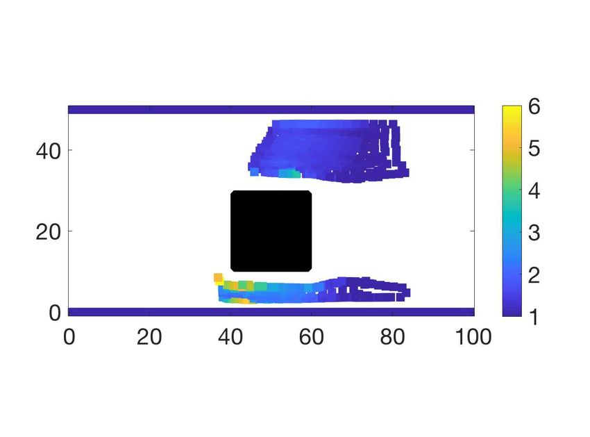
an Eikonal equation. This model is coupled with a non-local SEIS con-
      tagion model for disease spread, where besides the description of local
      contacts also the influence of contact times has been modelled. Hydro-
      dynamic approximations of the coupled system are derived. Finally,
      simulations of the hydrodynamic model are carried out using a mesh-
      free particle method. Different numerical test cases are investigated
      including uni- and bi-directional flow in a passage with and without
      obstacles.

  keywords:pedestrian flow models; disease spread models; multi-group
macroscopic equations; particle methods

    AMS Subject Classification:22E46, 53C35, 57S20

1    Introduction
The COVID-19 pandemic struck the everyday life worldwide. To avoid fur-
ther spread in absence of a vaccine or a well-established medical therapy,
most countries in the world invoked non-pharmaceutical intervention mea-
sures as extensive backtracking, testing and quarantine [21, 12]. One key
point is the contact reduction, which is often based on the minimization of
the number of contacts and contact time [1, 21, 47]. In many cases, such as
in schools or large working facilities social distancing is not always possible,
especially at the end of classes or shifts, crowds are formed to leave the fa-
cilities. Simulations of disease spread in a moving crowd could give valuable
information about how risky these mass events are and support the design
of such intervention measures.
     Modelling of crowd motion has been investigated in many works on dif-
ferent levels of description. Microscopic (individual-based) models based on
Newton type equations as well as vision-based models or cellular automata
models and agent-based models have been developed, see Refs. [24, 25, 11,
16, 38, 41]. Associated macroscopic pedestrian flow equations involving equa-
tions for density and mean velocity of the flow have been derived as well and
investigated thoroughly, see Refs. [6, 38, 23, 20, 2, 13, 14]. An elegant way to
include geometrical information and goal of the pedestrians into these mod-
els via the additional solution of an eikonal equation has been developed by
Hughes, see Refs. [2, 18, 28, 29, 35]. For the derivation and relations of the

                                        2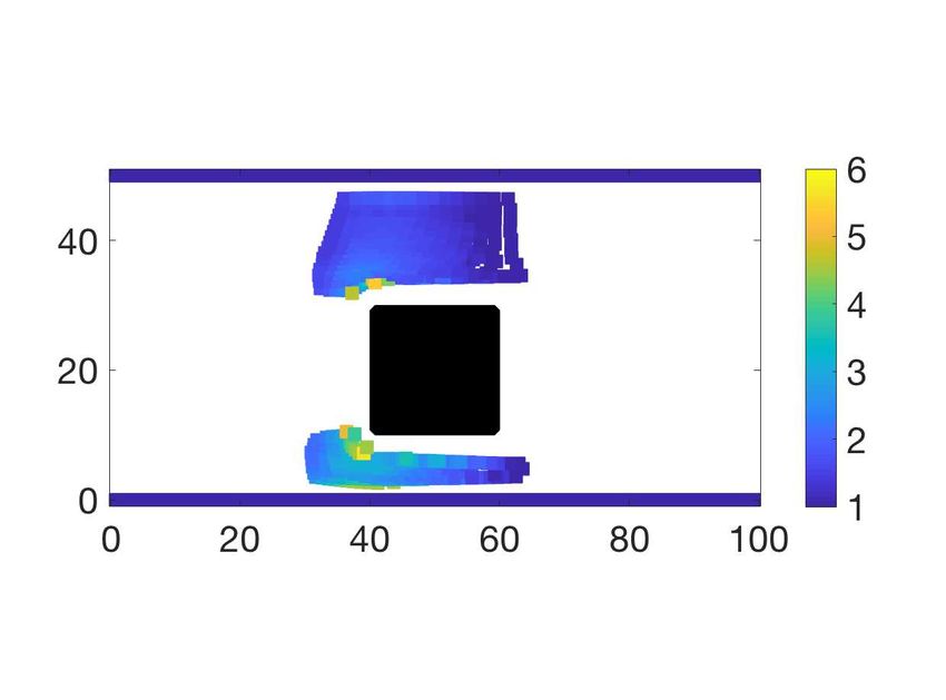
aboves approaches to each other we refer to Refs. [19, 15, 20]. More com-
plex geometries and obstacles have been included into the models by many
authors, see, for example, Refs. [41, 45, 46]. Pros and Cons of these models
have been discussed in various reviews, we refer to Refs. [6, 26, 3, 7] for a
detailed discussion of the different approaches.
    On the other hand, there is a vast literature on disease spread models,
see Ref. [5] for an overview on multiscale models and connection to crowd
dynamics. Moreover, we refer to Refs. [22, 34, 39, 17] for a small selection of
papers on mathematical models based on dynamical systems and to Refs. [27,
40, 9] for agent-based and network models. Models coupling crowd motion
and contagion dynamics are far less investigated. We refer to Ref. [31] for a
recent investigation coupling a crowd motion model with a contagion model
in a one-dimensional situation.
    One main objective of the present paper is to include a kinetic disease
spread model in the form of a multi-group equation into a kinetic pedestrian
dynamics model, derive hydrodynamic approximations and provide an effi-
cient numerical simulation of the coupled model for complex two-dimensional
geometries. For the pedestrian flow model we consider a kinetic equation for
multi-group pedestrian flow based on a social force model coupled with an
Eikonal equation to model geometry and goals of the pedestrians. This model
is coupled with a non-local contagion model for disease spread, where local
contacts as well as the influence of contact times is included. A second ob-
jective is the extension of the methodology to situations with more complex
geometries and moving objects in the computational domain. This is a way
to model, for example, the detailed interaction of pedestrians with larger
geometrically extended objects like cars in a shared space environment. See
[10] for another approach to the interaction of pedestrians and vehicles. The
numerical simulation is, as in Refs. [20, 33] , based on mesh-free particle
methods [43] for the solution of the Lagrangian form of the hydrodynamic
equations. Such a methodology gives an efficient and elegant way to solve
the full coupled problem in a complex environment.
    The paper is organized in the following way: in section 2 a kinetic model
for pedestrian dynamics with disease spread is presented. The section con-
tains also the associated hydrodynamic equations derived from a moment
closure approach. The meshfree particle methods used in the simulations is
shortly described in Section 3. The section contains also the results of the
numerical simulations. The solutions of the macroscopic equations are pre-
sented for different physical situations and parameter values including uni-

                                      3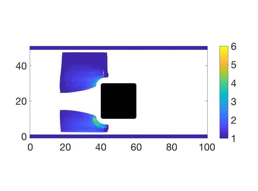
and bi-directional flow in a two-dimensional passage without obstacles and
with fixed and moving obstacles.

2      Equations
We use a kinetic model for the evolution of the distribution functions of
susceptible, exposed and infected pedestrians as a starting point and derive
associated hydrodynamic equations.

2.1     Kinetic evolution equation
We consider an equation for the evolution of pedestrian distribution functions
f (k) = f (k) (x, v, t), k = S, E, I. Here f S stands for the distribution of sus-
ceptible pedestrians, f E for the exposed pedestrians and f I for the infected.
The evolution equations are given by

                         ∂t f k + v · ∇x f k + Rf k = T k                     (1)

with k = S, E, I. The operators R and T k are given by the following defini-
tions.
            Rf k (x, v) = ∇v · [G(x, v; Φ, ρ) − ∇x U ⋆ ρ(x)]f k .


with
                                  ρ = ρS + ρE + ρI ,
where                                   Z
                              k
                             ρ (x) =        f k (x, v)dv.

Here, U is an interaction potential describing the local interaction of the
pedestrians and ⋆ denotes the convolution. Common choices for the inter-
action potential are purely repelling potentials like spring-damper potentials
or attractive-repulsive potentials like the Morse potential. In this paper we
have, for simplicity, considered a Morse potential without attraction given
by
                                           |x − y|
                           U = Cr exp −              ,                     (2)
                                              lr
where Cr is the repulsive strength and lr is the length scale. The part of the
forcing term involving G describes the influence of the geometry on the pedes-
trian’s motion and a potential long range interaction between the pedestrians,

                                            4
see below for a detailed description. The operators T k are defined using a
SEIS-type kinetic disease spread model leading to
T S = νf I − βI f S
T E = βI f S − θf E (3)
T I = θf E − νf I
with constants ν, θ, see Remark 3 below, and the non-local infection rate
βI = βI (x, v; f S (·), f E (·), f I (·)) depending in a non-local way on the rate of
infected persons, compare Refs. [31, 9] for similiar approaches. We define
1
Z Z
βI = φ(x − y, v − w)f I (y, w)dwdy. (4)
ρ(y)
The kernel φ in the infection rate is chosen as
φ = φ(x, v) = io φX (x)φV (v). (5)
R R
with φX (x)dx = 1 = φV (v)dv. Here, φX is determined as a decaying
function of |x| to take into account the effect that infections between pedes-
trians are more probable the closer pedestrians are approaching each other.
φV is chosen in a similar way depending on |v| to take into account the fact,
that infections are more probable the longer the interacting pedestrians stay
close to each other, that means the smaller their relative velocities are. The
parameter io is determined by the infectivity. We refer to the section on
numerical results for the exact definition of these kernels.
Finally, G is given by
1 ∇Φ(x)
G(x, v; Φ, ρ) = −V (ρ(x)) −v , (6)
T k∇Φ(x)k
where Φ is determined by the coupled solution of the eikonal equation
V (ρ)k∇Φk = 1. (7)
This describes the tendency of the pedestrians to move with a velocity given
by a speed V (ρ) and a direction given by the solution of the eikonal equa-
tion. The eikonal equation essentially includes all information about the
boundaries and the desired direction of the pedestrians via the boundary
conditions. These boundary conditions for the eikonal equation are chosen
5in the following way. For walls or for the boundaries of obstacles in the do-
main we set the value of Φ at the boundary to a numerically large value. For
ingoing boundaries, free boundary conditions for Φ are chosen, whereas for
outgoing boundaries, where the pedestrians aim to go, we set Φ = 0.
We note that on the one hand, the eikonal equation includes the geomet-
rical information via boundary conditions. On the other hand, it models a
global reaction of the pedestrians to avoid regions of dense crowds via the
term V (ρ) in (7).
Remark 1. The parameters in the above formulas, in particular in the def-
inition of (7) and (2) have to be chosen consistent with empirical data, see
[8, 30].
Remark 2. Instead of the social force model used here, one could as well
use more sophisticated interaction models, see for example [16, 4, 36]. We
note that the differences between these models in the present hydrodynamic
context are small. The behaviour of the solutions is rather dependent on the
choice of the parameters.
Remark 3. The dynamical system called the SEIS-model with constant in-
fection rate is given by
dS
= −βIS + νI
dt
dE
= βIS − θE
dt
dI
= θE − νI
dt
where β is the infection rate, ν the recovery rate and θ the rate with which
exposed persons are becoming infected. Pedestrians are potentially becoming
exposed, when they are in contact with infected pedestrians. However, ex-
posed pedestrians are only becoming infectious with a certain rate θ. Exposed
pedestrians do not infect other pedestrians. Usually, in the situations and on
the time scales under consideration here, ν and θ are very small and set to
zero in numerical simulations such that the number of infected pedestrians
remains constant during the simulation.
Remark 4. A key difference between other agent-based models as e.g. [9] is
the dependence of the infection on the relative velocity of the agents. This
has direct implications on the process of infection during the dynamics, as
can be seen the the case studies.
62.2 The multi-group hydrodynamic model
Integrating the kinetic equation against dv and vdv and using a mono-kinetic
distribution function to close the resulting balance equations, i.e. approxi-
mate
f k ∼ ρk (x)δu(x) (v)
one obtains a continuity equation for group k
Z
∂t ρ + ∇x · (ρ u) = T k dv
k k
(8)
and the momentum equation
∂t u + (u · ∇x )u = G(x, u; Φ, ρ) − ∇x U ⋆ ρ (9)
with the total density ρ given as
ρ = ρS + ρE + ρI .
Moreover,
1 ∇Φ(x)
G(x, u; Φ, ρ) = −V (ρ(x)) −u ,
T k∇Φ(x)k
where Φ is determined by solving the eikonal equation
V (ρ)k∇Φk = 1.
The continuity equations are explicitly written as
∂t ρS + ∇x · (uρS ) = νρI − βI ρS
∂t ρE + ∇x · (uρE ) = βI ρS − θρE (10)
∂t ρI + ∇x · (uρI ) = θρE − νρI .
with βI = βI (x; ρS (·), ρE (·), ρI (·), u(·)), where now
ρI (y)
Z
βI = φ(x − y, u(x) − u(y)) dy. (11)
ρ(y)
Remark 5. Multi-group models for pedestrian flows have been also used in
different contexts. For example in [37] a hydrodynamic multi-group model
for pedestrian dynamics with groups of different sizes has been developed and
analysed in [37].
72.3 The hydrodynamic model using volume fractions
For numerical computations this is rewritten using volume fractions, that
means we solve the continuity equation
∂t ρ + ∇x · (ρu) = 0 (12)
and the momentum equation
∂t u + (u · ∇x )u = G(x, u; Φ, ρ) − ∇x U ⋆ ρ. (13)
Then we compute the volume fractions αS , αE , αI with αS + αE + αI = 1
as
∂t αS + u · ∇x αS = ναI − β I αS
∂t αE + u · ∇x αE = β I αS − θαE (14)
∂t αI + u · ∇x αI = θαE − ναI
with βI = βI (x; αI (·), u(·)) defined by
Z
βI = φ(x − y, u(x) − u(y))αI (y)dy. (15)
Finally, one computes
ρI = αI ρ, ρS = αS ρ, ρE = αE ρ.
2.4 Dynamic geometries
We allow the domain on which the above equations are defined to depend on
time. In particular, we consider moving obstacles, which change their path
and speed in order to avoid collisions with the pedestrians, while moving
towards a specific target. The interaction between the pedestrians and the
moving obstacle is additionally modeled by kinematic equations using a re-
pulsive potential similar to the pedestrian-pedestrian interactions. A second
Eikonal equation is integrated for modelling the path of the moving obstacle
in the geometry and the desired destination of the obstacle. The velocity
update equation for the obstacle is given as
dxO
= vO ,
dt
8dv O
= −∇x U O ∗ ρ(xO ) + GO (xO , v O ; ΦO , ρ) , (16)
dt
where xO and v O are the position and velocity of the obstacle’s centre of
mass, ρ is the density of pedestrians at xO . U O is an interaction potential
describing the interaction of the pedestrians on the obstacle.
GO is obtained from the gradient of the Eikonal solution φO for the ob-
stacle as
∇φO (xO )
O O O O 1 O O O
G (x , v ; Φ , ρ) = − O −V (ρ(x )) −v , ||∇φO || = 1.
T ||∇φO (xO )||
That means, the eikonal equation is for the obstacle only used to include
the geometrical informations and the goal of the obstacle. We note that the
action of the obstacle on the pedestrians is given by the solution of equation
(7) via the boundary conditions at the obstacle’s boundaries. In contrast,
the action of the pedestrians on the obstacle is given via U O .
3 Numerical method and results
For the numerical simulation we use a meshfree particle method, which is
based on least square approximations. [44, 33] A Lagrangian formulation of
the hydrodynamic equations is used and coupled to the SEIS model and the
obstacle’s kinematic equations Eq. (16).
3.1 Lagrangian equations
The spatially discretizted system in Lagrangian form is given by
dxi
= ui ,
dt
dρi
= −ρi ∇x · ui ,
dt
dui X
= G(xi , ui ; Φ, ρ) − ∇U(xi − xj )ρj dVj ,
dt j
(17)
and
dαiS
= ναiI − βiI αiS (18)
dt
9dαiE
= βiI αiS − θαiE (19)
dt
dαiI
= θαiE − ναiI (20)
dt
with X
βiI = φ(xi − xj , ui − uj ) αjI dVj ,
j
and
dxO
= vO ,
dt
dv O X
= GO (xO , v O ; ΦO , ρ) − ∇U O (xO − xj )ρj dVj . (21)
dt j
Here dVj is the local area around a particle.
Remark 6. Although the equations in Lagrangian form look similiar to a
microscopic problem, there are important differences. In particular, the effi-
cient solution of the continuity equation (compared to a determination of the
density in a purely microscopic simulation) and the consequent availablity of
ρi on each grid-point allows the efficient use of the density, used at various
places in the model.
3.2 Numerical method
For a description of the mesh-free method for the pedestrian flow equations
in a fixed rectangular domain, we refer to [43, 33]. There, the eikonal equa-
tion has been solved on a separate regular mesh on the entire domain using
the fast-marching method. The information from the irregular point cloud,
used for solving the fluid equations has been interpolated to the eikonal grid
and vice versa. Such an approach requires for a moving obstacle to take
special care of the grid points being overlapped by the obstacles. Using an
immersed boundary method, they are activated and deacitvated depending
on the location of the obstacle.
Here, we have followed a different approach. The eikonal equation is
directly solved on the irregular point cloud used for the hydrodynamic equa-
tions. Thus, in each time step an eikonal equation on an unstructured grid
has to be solved, see [42] for the Fast-marching method in this case. The
10approximation of the spatial derivatives in the eikonal equation is obtained
as for the hydrodynamic equations: the spatial derivatives at an arbitrary
grid point are computed from the values at its surrounding neighboring grid
points using a weighted least squares method. We refer to [32] for a numer-
ical study of the accuracy and complexity of such a method for the eikonal
equation.
Finally, we note that for a uni-directional flow of pedestrians, we have
to solve only one eikonal equation. If there is bi-directional flow, we have
to solve an eikonal equation for each direction. The same would be true for
several obstacles with different goals.
3.3 Numerical results
We have performed numerical simulations of equations (Eq. (12) to Eq. (15)
and (16) for different scenarios. In all our simulations, we consider a com-
putational domain given by a platform or corridor of size 100 m × 50 m.
The top and bottom boundaries are rigid walls without any entry or exit.
Right and left boundary are exits for pedestrians and obstacles depending on
the situation under consideration. We consider uni- as well as bi-directional
flow of the pedestrians. Initially, the pedestrians are distributed as shown in
Figure 1 with a distance of 1.575m from each other. We consider the cases
with and without obstacles, which are either fixed or moving. We initialize
the infected pedestrians (colored in red) with αI = 1, αS = 0, αE = 0, the
susceptibles (in green) by αI = 0, αS = 1, αE = 0.
4
We have used for the infection rate βI the functions φX =exp(−|x − y| )
ρ
and φV = exp(−|u − v|6 ). Moreover, we choose V (ρ) = Vmax 1 − ρmax and
V O (ρ) in the same way with Vmax substitued by Vmax
O
. For the parameters
we have used the values given in Table 1.
Variable Value Variable Value
Vmax 2 m/s ρmax 10 ped/m2
O
Vmax 3 m/s T 0.001 s
Cr = CrO 50 lr 2m
lrO 1m io 0.04 m2 /s2
Table 1: Numerical parameters.
11100
100
80
80
60
60
40
40
20
20
0
0
50
40
30
20
10
50
40
30
20
10
0
0
100
100
80
80
60
60
40
40
20
20
0
0
50
40
30
20
10
0
50
40
30
20
10
0
Figure 1: Initial situation at t = 0. Top row: Uni-directional (left) and
bi-directional (right) flow. Bottom row: Fixed obstacle (left) and moving
obstacle (right). Red indicate infected, green indicate susceptible pedestri-
ans.
12During the evolution, infected pedestrians are colored in red, susceptibles
in green and exposed pedestrians in blue according to the values of αk . If
αE > 0.05 the colour is switching from green to blue, meaning that the proba-
bility of being exposed has exceeded a certain threshold. The red pedestrians
remain red throughout the simulations, since the recovery rate ν is set equal
to 0 in the simulations. Moreover, since θ is also set to 0 exposed patients
are not becoming infected and cannot infect others in the simulations.
The fixed and the moving obstacle considered are rectangular in shape
and initially located as shown in Figure 1.
Explicit time integration of the equations in Lagrangian form is done with
a fixed time step size of 0.001 in our simulations.
3.4 Test-case 1: fixed obstacle
In this first test case we have considered a fixed obstacle and compared
the results to a situation without obstacle. We consider bi-directional flow
without an obstacle and uni- and bi-directional flow with an obstacle. This
is done for the case φv = 0 (no influence of contact time) and the case where
φV is chosen as defined above, that means for a situation where the influence
of the contact time is included. The present initial configuration is chosen
in such a way, that there is no increase of the number of probably exposed
pedestrians, if a uni-directional flow without obstacle is considered with or
without influence of the contact time.
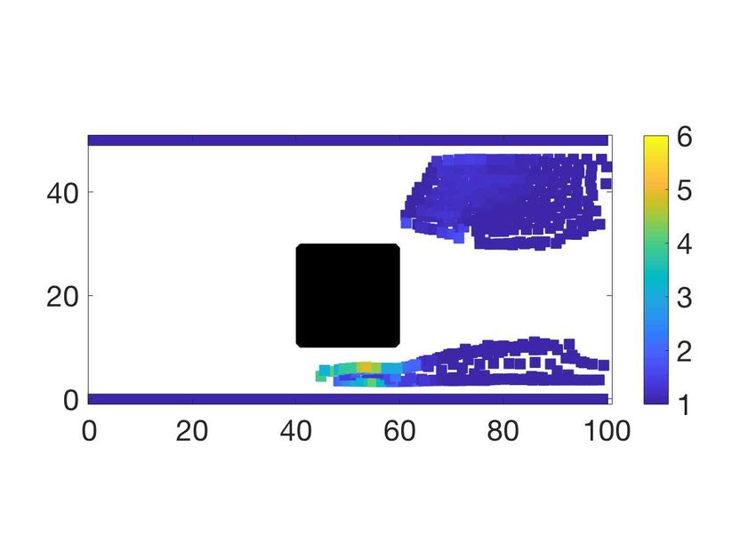
Figures 2 to 5 show the time evolution of the moving grid points and the
associated infection labels with influence (left column) and without influence
(right column) of contact time. Row 1 shows bi-directional flow without
an obstacle, row 2 shows uni-directional flow around an obstacle and row 3
shows bi-directional flow around an obstacle. Red indicate infected, green
indicate susceptibles and blue indicate exposed pedestrians.
Here one observes, e.g. in Figure 4 or 5, that in situations with bi-
directional flow (top- and bottom row), the number of exposed patients is
strongly reduced, if the contact time is taken into account. For uni-directional
flow, the differences are much smaller as expected, since pedestrians stay near
to each other for a longer time during the evolution.
Comparing row 2 (uni-dirctional with obstacle) with the uni-directional
case without obstacle (no exposed pedestrians), one observes that the number
of exposed patients is considerably increased due to the denser pedestrian
crowd surrounding the obstacle. Similar observations can be made comparing
13row 1 and row 3.
In Figure 6 we have plotted the number of pedestrians with a higher
probability of being exposed versus time. One can observe, that the number
of these pedestrians is much higher if the influence of the contact time is
neglected. This happens mainly in bi-directional flows, which is as expected,
since, even if pedestrians are coming close to each other, they pass each
other quickly and the contact time is short such that a contagion is less
probable. On the other hand if pedestrians are walking in the same direction,
the effect of neglecting the contact time is comparably small. We mention,
that the contagion model is based on very simple assumptions and obviously
the parameters of the contagion model have to be adapted to experimental
findings. We refer again to [31] for similiar investigations.
Finally, in Figure 7 we show the macroscopic density of the pedestrians
at times t = 10, 20, 30, 40 for the situation with influence of contact time for
uni-directional flow with fixed obstacle.
3.5 Test-case 2: moving obstacle
In this subsection we consider the interaction of pedestrians with a moving
obstacle, e.g. a vehicle in a shared space. We consider the same computa-
tional domain as in test-case 1 with pedestrians, which are initially located as
in Figure 1 (right bottom). Their destination is the right exit. The moving
obstacle of size 4m × 8m is located on the right with the left exit as destina-
tion. Typically in a restricted traffic area the vehicle has a low speed limit.
We have chosen 10km/h ∼ 3m/s. The maximum speed of the pedestrians is
chosen as 2m/s.
In Figure 8 we have plotted the positions of pedestrians and obstacle
at different times t = 8s, 14s, 18s and 22s. We observe an interaction of
pedestrians and obstacle between times t = 14s and t = 22s. Moreover,
one observes a slight increase of the number of exposed people which is less
pronounced than in the case of the big fixed obstacle in test-case 1.
Moreover, in Figure 9 we have plotted the x-velocity component of the
obstacle along its center of mass. One observes that the obstacle (coming
from the right) accelerates and maintains almost its maximum speed. When
it encounters the pedestrian crowd, it reduces its speed. Finally, it accelerates
again, when there are no pedestrians anymore in the surroundings.
1450 50
40 40
30 30
20 20
10 10
0 0
20 40 60 80 100 0 20 40 60 80 100 0 20 40 60 80 100
15
50 50
40 40
30 30
20 20
10 10
0 0
20 40 60 80 100 0 20 40 60 80 100 0 20 40 60 80 10050 50
40 40
30 30
20 20
10 10
0 0
20 40 60 80 100 0 20 40 60 80 100 0 20 40 60 80 100
16
50 50
40 40
30 30
20 20
10 10
0 0
20 40 60 80 100 0 20 40 60 80 100 0 20 40 60 80 10050 50
40 40
30 30
20 20
10 10
0 0
20 40 60 80 100 0 20 40 60 80 100 0 20 40 60 80 100
17
50 50
40 40
30 30
20 20
10 10
0 0
20 40 60 80 100 0 20 40 60 80 100 0 20 40 60 80 10050 50
40 40
30 30
20 20
10 10
0 0
20 40 60 80 100 0 20 40 60 80 100 0 20 40 60 80 100
18
50 50
40 40
30 30
20 20
10 10
0 0
20 40 60 80 100 0 20 40 60 80 100 0 20 40 60 80 10040
40
30
30
Time (t)
Time (t)
20
20
= exp(-|u-v| 6)
)
= exp(-|u-v|
=1
10
10
=1
V
V
V
V
0
0
12
10
25
20
15
10
8
6
4
2
0
5
0
No. of exposed pedestrian (in %) No. of exposed pedestrian (in %)
40
30
Time (t)
20
= exp(-|u-v| )
6
10
=1 V
V
0
8
6
4
2
0
No. of exposed pedestrian (in %)
Figure 6: Number of pedestrian with an increased probablity of being ex-
posed (in %) vs time. First row bi-directional flow without obstacle (left)
and with obstacle (right). Second row: uni-directional with obstacle.
19Figure 7: Macroscopic density ρ of pedestrian dynamics at times t =
10, 20, 30, 40 with influence of contact time for uni-direction flow with fixed
obstacle.
20100
100
80
80
60
60
40
40
20
20
0
0
50
40
30
20
10
50
40
30
20
10
0
0
100
100
80
80
60
60
40
40
20
20
0
0
50
40
30
20
10
50
40
30
20
10
0
0
Figure 8: Positions of pedestrian and obstacle at t = 8s, 14s (first row) and
t = 18s, 22s (second row). Red indicate infected, green indicate susceptibles,
blue indicate probably exposed pedestrians.
21100
80
Center of mass
40
20
0 60
0
-0.5
-1
-1.5
-2
-2.5
-3
X-velo. comp. of obstacle
Figure 9: The velocity of the obstacle along the center of mass.
224 Concluding Remarks
We have presented a multi-group macroscopic pedestrian flow model combin-
ing a dynamic model for pedestrians flows and a SEIS based kinetic disease
spread model. A meshfree particle method to solve the governing equations is
presented and used for the computation of several numerical examples analyz-
ing different situations and parameters. The dependence of the solutions and,
in particular, the dependence of the number of exposed pedestrians on ge-
ometry and parameters is investigated and discussed and shows qualitatively
consistent results. Findings indicate, that in particular, in bi-directional flow
it is important to take into account the contact time for a realistic description
of the flow. This is a realistic qualitative behavior, which sheds a new light
for the design of emergency exits in the presence of a pandemic.
Acknowledgment
This work is supported by the German research foundation, DFG grant KL
1105/30-1 and by the DAAD PhD program MIC.
References
[1] B. Adamik, M. Bawiec, V. Bezborodov, W. Bock, M. Bodych , J. Bur-
gard, ... & T. Ozanski, (2020). Mitigation and herd immunity strategy for
COVID-19 is likely to fail. medRxiv (preprint) Available at: https://doi.
org/10.1101/2020.03, 25.
[2] D. Amadoria and M. Di Francesco, The one-dimensional Hughes model
for pedestrian flow: Riemann-type solutions, Acta Math. Sci. 32 (2012)
259-280.
[3] G. Albi, N. Bellomo, L. Fermo, S.-Y. Ha, J. Kim, L. Pareschi, D. Poyato,
and J. Soler, Traffic, crowds, and swarms. From kinetic theory and mul-
tiscale methods to applications and research perspectives, Math. Models
Methods Appl. Sci., 29, (2019), 1901-2005.
[4] R. Bailo, J. A. Carrillo, P. Degond, Pedestrian Models based on Rational
Behaviour, https://arxiv.org/abs/1808.07426
23[5] N. Bellomo, R. Bingham, M. A. J. Chaplain, G. Dosi, G. Forni, D. A.
Knopoff, J. Lowengrub, R. Twarock, and M. E. Virgillito, A multi-
scale model of virus pandemic: Heterogeneous interactive entities in
a globally connected world, Math. Models Methods Appl. Sci., doi:
10.1142/S0218202520500323.
[6] N. Bellomo and C. Dogbe, On the modeling of traffic and crowds: A
survey of models, speculations, and perspectives, SIAM Rev. 53 (2011)
409-463.
[7] N. Bellomo, A. Bellouquid, D. Knopoff, From the microscale to collective
crowd dynamics, SIAM J. Multiscale Model. Simul. 11 (2013) 943–963.
[8] N. Bellomo, L. Gibelli, and N. Outada, On the Interplay between Be-
havioral Dynamics and Social Interactions in Human Crowds, Kinetic
Related Models, 12, (2019), 397-409, (2019).
[9] W. Bock, T. Fattler, I. Rodiah, and O.Tse. An analytic method for
agent-based modeling of spatially inhomogeneous disease dynamics. In
AIP Conference Proceedings (Vol. 1871, No. 1, p. 020008). AIP Pub-
lishing LLC. 2017.
[10] R. Borsche, A. Klar, S. Kühn, A. Meurer, Coupling traffic flow networks
to pedestrian motion, Math. Methods Models Appl. Sci. 24, 2, 359-380,
2014
[11] C. Burstedde, K. Klauck, A. Schadschneider, J. Zittartz, Simulation of
pedestrian dynamics using a two-dimensional cellular automaton, Phys-
ica A 295 507–525, 2001.
[12] R.Chowdhury, K.Heng, M. S. R. Shawon, G. Goh, D. Okonofua, C.
Ochoa-Rosales, ... & S. Shahzad (2020). Dynamic interventions to con-
trol COVID-19 pandemic: a multivariate prediction modelling study
comparing 16 worldwide countries. European journal of epidemiology,
35(5), 389-399.
[13] R. Colombo, M. Garavello, M. Lecureux-Mercier, A Class of Non-Local
Models for Pedestrian Traffic, Math. Models Methods Appl. Sci. 22
(2012) 1150023.
24[14] R. Colombo, M. Garavello, M. Lecureux-Mercier, Non-local crowd dy-
namics, Comptes Rendus Mathmatique 349 (2011) 769–772.
[15] E. Cristiani, B. Piccoli, and A. Tosin, Multiscale Modeling of Pedestrian
Dynamics, Springer, (2014).
[16] P. Degond, C. Appert-Rolland, M. Moussaid, J. Pettre and G. Ther-
aulaz, A hierarchy of heuristic-based models of crowd dynamics, J. Stat.
Phys. 152 (2013) 1033-1068.
[17] Dessalegn Y. Melesse, Abba B. Gumel, Global asymptotic properties of
an SEIRS model with multiple infectious stages, J. Math. Anal. Appl.
366 (2010) 202–217.
[18] M. Di Francesco, P.A. Markowich, J.F. Pietschmann and M.T. Wolfram,
On the Hughes model for pedestrian flow: The one-dimensional case, J.
Differential Equations 250 (2011) 1334-1362.
[19] M. Di Francesco, S. Fagioli, M.D. Rosini, G. Russo, Deterministic parti-
cle approximation of the Hughes model in one space dimension, Kinetic
and Related Models, 10, 1, (2017), 215–237
[20] R Etikyala, S Göttlich, A Klar, and S Tiwari. Particle methods for
pedestrian flow models: From microscopic to nonlocal continuum models
Mathematical Models and Methods in Applied Sciences, 20(12), 2503–
2523, 2014.
[21] N.M.Ferguson , D. Laydon, G. Nedjati-Gilani, et al. Impact of non-
pharmaceutical interventions (NPIs) to reduce COVID19 mortality and
healthcare demand. London: WHO Collaborating Centre for Infectious
Disease Modelling MRC Centre for Global Infectious Disease Analysis
Abdul Latif Jameel Institute for Disease and Emergency Analytics Im-
perial College London; 2020.
[22] Herbert W. Hethcote, The Mathematics of Infectious Diseases, SIAM
REVIEW Vol. 42, No. 4, pp. 599–653, 2000
[23] D. Helbing, A fluid dynamic model for the movement of pedestrians,
Complex Syst. 6 (1992) 391-415.
25[24] D. Helbing and P. Molnar, Social force model for pedestrian dynamics,
Phys. Rev. E, 51 (1995), pp. 4282-4286.
[25] D. Helbing, I.J. Farkas, P. Molnar, and T. Vicsek, Simulation of pedes-
trian crowds in normal and evacuation situations, in: M. Schreckenberg,
S.D. Sharma(Eds.), Pedestrian and Evacuation Dynamics, Springer-
Verlag, Berlin, 2002, pp. 21-58.
[26] D. Helbing, A. Johansson, Pedestrian, Crowd and Evacuation Dynamics.
Encyclopedia of Complexity and Systems Science 16, (210), 6476-6495.
[27] T. House, Modelling epidemics on networks. Contemporary Physics,
53(3), pp.213-225, 2012.
[28] R.L. Hughes, A continuum theory for the flow of pedestrians, Transp.
Res. Part B: Methodological 36 (6) (2002), pp. 507-535.
[29] R.L. Hughes, The flow of human crowds, Ann. Rev. Fluid Mech. 35
(2003) 169-182.
[30] D.P. Kennedy, J. Gläscher, J.M. Tyszka, R. Adolphs, Personal space
regulation by the human amygdala. Nat Neurosci. 12, 1226–1227, 2009.
[31] D. Kim and A. Quaini, Coupling kinetic theory approaches for pedes-
trian dynamics and disease contagion in a confined environment, Math.
Models Methods Appl. Sci., 30(9), (2020).
[32] A. Klar, S. Tiwari, and E. Raghavender, Mesh Free method for Nu-
merical Solution of The Eikonal Equation, Proceedings of International
workshop on PDE Modelling and Computation, Advances in PDE Mod-
elling and Computation, Ane Books Pvt. Ltd., 2013.
[33] A. Klar, S. Tiwari, A multi-scale particle method for mean field equa-
tions: the general case, SIAM Multiscale Mod. Simul. 17 (1), 233-259,
2019
[34] Andrei Korobeinikov, Lyapunov functions and global properties for SEIR
and SEIS epidemic models, Mathematical Medicine and Biology, 2004
26[35] H. Ling, S.C. Wong, M. Zhang, C.H. Shu, and W.H.K. Lam, Revisiting
Hughes dynamics continuum model for pedestrian flow and the develop-
ment of an efficient solution algorithm, Transp. Res. Part B: Method-
ological, 43 (1) (2009), pp. 127-141.
[36] N. K. Mahato, A. Klar, S. Tiwari, A meshfree particle method for
a vision-based macroscopic pedestrian model, Int. J. Adv. Eng. Sci.
Appl.Math 10, 1, 41-53, 2018
[37] N.K. Mahato, A. Klar, S. Tiwari, Particle methods for multi-group pedes-
trian flow, Appl. Math. Modeling 53, 447-461, 2018
[38] B. Maury, A. Roudneff-Chupin and F. Santambrogio, A macroscopic
crowd motion model of the gradient-flow type, Math. Models Methods
Appl. Sci. 20 (2010) 1787-1921.
[39] Suzanne M. O’Regan, Thomas C. Kelly, Andrei Korobeinikov, Michael
J.A. O’Callaghan, Alexei V. Pokrovskii, Lyapunov functions for SIR and
SIRS epidemic models, AppliedMathematicsLetters23, 446–448, 2010
[40] L. Perez, & S. Dragicevic, An agent-based approach for modeling dy-
namics of contagious disease spread. International journal of health ge-
ographics, 8(1), 50, 2009.
[41] B. Piccoli and A. Tosin, Pedestrian flows in bounded domains with ob-
stacles, Contin. Mech. Thermodynam. 21 (2009) 85-107.
[42] J.A. Sethian, Fast marching methods, SIAM Rev. 41 (1999) 199-235.
[43] S. Tiwari, and J. Kuhnert, Finite pointset method based on the projection
method for simulations of the incompressible Navier-Stokes equations,
Meshfree Methods for Partial Differential Equations, eds. M. Griebel
and M.A. Schweitzer, Lecture Notes in Computational Science and En-
gineering, Vol. 26 (Springer-Verlag, 2003), pp. 373-387.
[44] S. Tiwari, and J. Kuhnert, Modelling of two-phase flow with surface ten-
sion by finite pointset method(FPM), J. Comp. Appl. Math, 203 (2007),
pp. 376-386.
[45] M. Twarogowska, P. Goatin, R. Duvigneau, Macroscopic modeling and
simulations of room evacuation, Applied Mathematical Modelling, 38,
Issue 24, 2014, 5781-5795
27[46] A. Treuille, S. Cooper, Z. Popovic, Continuum crowds, in: ACM Trans-
action on Graphics, Proceedings of SCM SIGGRAPH 25 (2006) 1160–
1168.
[47] P.G. Walker, C. Whittaker, O. Watson, et al. The global impact of
COVID-19 and strategies for mitigation and suppression. London: WHO
Collaborating Centre for Infectious Disease Modelling, MRC Centre for
Global Infectious Disease Analysis, Abdul Latif Jameel Institute for Dis-
ease and Emergency Analytics, Imperial College London; 2020.
28You can also read