The Development of an Instrument for Longitudinal Learning Diagnosis of Rational Number Operations Based on Parallel Tests - Frontiers
←
→
Page content transcription
If your browser does not render page correctly, please read the page content below
ORIGINAL RESEARCH
                                                                                                                                      published: 02 September 2020
                                                                                                                                     doi: 10.3389/fpsyg.2020.02246

                                            The Development of an Instrument
                                            for Longitudinal Learning Diagnosis
                                            of Rational Number Operations
                                            Based on Parallel Tests
                                            Fang Tang and Peida Zhan*
                                            Department of Psychology, College of Teacher Education, Zhejiang Normal University, Jinhua, China

                                            The precondition of the measurement of longitudinal learning is a high-quality
                                            instrument for longitudinal learning diagnosis. This study developed an instrument for
                                            longitudinal learning diagnosis of rational number operations. In order to provide a
                                            reference for practitioners to develop the instrument for longitudinal learning diagnosis,
                                            the development process was presented step by step. The development process
                                            contains three main phases, the Q-matrix construction and item development, the
                                            preliminary/pilot test for item quality monitoring, and the formal test for test quality
                         Edited by:         control. The results of this study indicate that (a) both the overall quality of the tests
                         Liu Yanlou,
                                            and the quality of each item are good enough and that (b) the three tests meet the
        Qufu Normal University, China
                                            requirements of parallel tests, which can be used as an instrument for longitudinal
                         Reviewed by:
                          Wenyi Wang,       learning diagnosis to track students’ learning.
      Jiangxi Normal University, China
                                Ren Liu,    Keywords: learning diagnosis, longitudinal assessments, rational number operations, parallel tests, longitudinal
                                            cognitive diagnosis
      University of California, Merced,
                          United States
                  *Correspondence:
                         Peida Zhan
                                            INTRODUCTION
                  pdzhan@gmail.com
                                            In recent decades, with the development of psychometrics, learning diagnosis (Zhan, 2020b)
                   Specialty section:
                                            or cognitive diagnosis (Leighton and Gierl, 2007), which objectively quantifies students’ current
         This article was submitted to      learning status, has drawn increasing interest. Learning diagnosis aims to promote students’
              Quantitative Psychology       learning according to diagnostic results which typically including diagnostic feedback and
                    and Measurement,        interventions. However, most existing cross-sectional learning diagnoses are not concerned about
               a section of the journal     measuring growth in learning. By contrast, longitudinal learning diagnosis evaluates students’
               Frontiers in Psychology      knowledge and skills (collectively known as latent attributes) and identifies their strengths and
            Received: 06 July 2020          weaknesses over a period (Zhan, 2020b).
        Accepted: 11 August 2020               A complete longitudinal learning diagnosis should include at least two parts: an instrument
     Published: 02 September 2020
                                            for longitudinal learning diagnosis of specific content and a longitudinal learning diagnosis model
                             Citation:      (LDM). The precondition of the measurement of longitudinal learning is a high-quality instrument
        Tang F and Zhan P (2020) The        for longitudinal learning diagnosis. The data collected from the instrument for longitudinal
        Development of an Instrument
                                            learning diagnosis can provide researchers with opportunities to develop longitudinal LDMs
   for Longitudinal Learning Diagnosis
of Rational Number Operations Based
                                            that can be used to track individual growth over time. Additionally, in recent years, several
                      on Parallel Tests.    longitudinal LDMs have been proposed, for review, see Zhan (2020a). Although the usefulness
              Front. Psychol. 11:2246.      of these longitudinal LDMs in analyzing longitudinal learning diagnosis data has been evaluated
       doi: 10.3389/fpsyg.2020.02246        through some simulation studies and a few applications, the development process of an instrument

Frontiers in Psychology | www.frontiersin.org                                     1                                       September 2020 | Volume 11 | Article 2246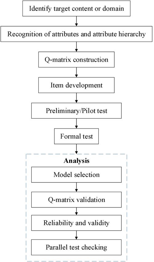
Tang and Zhan                                                                                            An Instrument for Longitudinal Learning Diagnosis

for longitudinal learning diagnosis is rarely mentioned (cf.
Wang et al., 2020). The lack of an operable development
process of instrument hinders the application and promotion
of longitudinal learning diagnosis in practice and prevents
practitioners from specific fields to apply this approach to track
individual growth in specific domains.
   Currently, there are many applications use cross-sectional
LDMs to diagnose individuals’ learning status in the field of
mathematics because the structure of mathematical attributes is
relative clear to be identified, such as fraction calculations
(Tatsuoka, 1983; Wu, 2019), linear algebraic equations
(Birenbaum et al., 1993), and spatial rotations (Chen et al.,
2018; Wang et al., 2018). Some studies also apply cross-sectional
LDMs to analyze data from large-scale mathematical assessments
(e.g., George and Robitzsch, 2018; Park et al., 2018; Zhan et al.,
2018; Wu et al., 2020). However, most of these application
studies use cross-sectional design and cannot track the individual
growth of mathematical ability.
   In the field of mathematics, understanding rational numbers
is crucial for students’ mathematics achievement (Booth
et al., 2014). Rational numbers and their operations are one
of the most basic concepts of numbers and mathematical
operations, respectively. The fact that many effects are put
into rational number teaching makes many students and
teachers struggle to understand rational numbers (Cramer
et al., 2002; Mazzocco and Devlin, 2008). The content of
rational number operation is the first challenge that students
encounter in the field of mathematics at the beginning
of junior high school. Learning rational number operation
is not only the premise of the subsequent learning of
mathematics in junior high school but is also an important
opportunity to cultivate students’ interest and confidence in
mathematics learning.
   The main purpose of this study is to develop an instrument
for longitudinal learning diagnosis, especially for the content of
rational number operations. We present the development process
step by step to provide a reference for practitioners to develop the        FIGURE 1 | The development process of the instrument for longitudinal
instrument for longitudinal learning diagnosis.                             learning diagnosis.

DEVELOPMENT OF THE INSTRUMENT                                              the confirmation of attributes mainly adopted the method
                                                                           of literature review (Henson and Douglas, 2005) and expert
FOR LONGITUDINAL LEARNING
                                                                           judgment (Buck et al., 1997; Roduta Roberts et al., 2014; Wu,
DIAGNOSIS                                                                  2019). This study used the combination of these two methods.
                                                                               First, relevant content knowledge was extracted according to
As the repeated measures design is not always feasible
                                                                           the analysis of mathematics curriculum standards, mathematics
in longitudinal educational measurement, in this study, the
                                                                           exam outlines, teaching materials and supporting books, existing
developed instrument is a longitudinal assessment consisting
                                                                           provincial tests, and chapter exercises. By reviewing the
of parallel tests. The whole development process is shown in
                                                                           literature, we find that the existing researches mainly focus
Figure 1. In the rest of the paper, we describe the development
                                                                           on one or several parts of rational number operation. For
process step by step.
                                                                           example, fraction addition and subtraction is the most involved
                                                                           in existing researches (e.g., Tatsuoka, 1983; Wu, 2019). In
Recognition of Attributes and Attribute                                    contrast, it is not common to focus on the whole part of
Hierarchy                                                                  rational number operation in diagnostic tests. Ning et al.
The first step in designing and developing a diagnostic assessment         (2012) pointed out that rational number operation contains 15
is recognizing the core attributes involved in the field of study          attributes; however, such a larger number of attributes does not
(Bradshaw et al., 2014). In the analysis of previous studies,              apply in practice.

Frontiers in Psychology | www.frontiersin.org                          2                                       September 2020 | Volume 11 | Article 2246
Tang and Zhan An Instrument for Longitudinal Learning Diagnosis
TABLE 1 | Attribute framework of the rational number operation. TABLE 2 | Items in think-aloud protocol analysis (original items are written
in Chinese).
Label Attribute Description
Please say out aloud your thoughts when you solve the problem.
A1 Rational number Concepts and classifications
(1) Which one of the following statement about rational numbers is correct? ().
A2 Related concepts of the Opposite number, absolute value
(A) Rational numbers can be divided into two categories: positive rational
rational number
numbers and negative rational numbers
A3 Number axis Concept, number conversion,
(B) The set of positive integers and the set of negative integers together
comparison of the size of numbers
constitute the set of integers
A4 Addition and subtraction of Addition, subtraction, and addition
(C) Integers and fractions are collectively called rational numbers
rational numbers operation rules
(D) Positive numbers, negative numbers, and zeros are collectively called
A5 Multiplication and division of Multiplication, involution, multiplication
rational numbers
rational numbers operation rule, division and reciprocal;
Reduction of fractions to a common (2) Which rational number’s inverse equals to itself? ().
denominator (A) () 1 (B) −1 (C) 0 (D) 0 and 1
A6 Mixed operation of rational First involution, then multiplication and
numbers division, and finally addition and (3) On the number axis, point A indicates −1. Now A starts to move, first move 3
subtraction; if there are numbers in units to the left, then 9 units to the right, and 5 units to the left. At this time, what
parentheses, calculate the ones in the the number is point A indicates? ().
parentheses first. (A) −1 (B) 0 (C) 1 (D) 8
(4) Computing: 9 + (−13) − (−7) + (−5) =
(5) Computing: (−2) × 14 ÷ (− 71 ) × (−1)5 =
(6) Computing: (− 25 ) × (− 37 ) − 2
7 − 3
5 ÷ (− 73 ) =
performance, gender balance, willingness to participate, and
ability to express their thinking process (Gierl et al., 2008). The
experimenter individually tested these students and recorded
their responses; in the response process, the students were
required to say aloud their problem-solving train of thought.
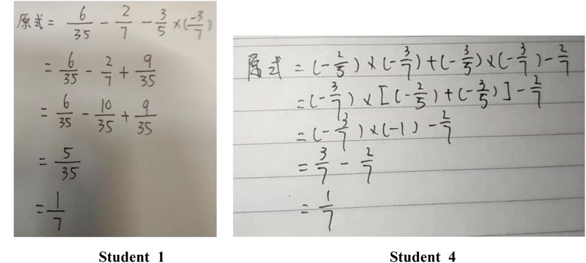
Taking the responses of two students to item 6 as an
example, Figure 3 and Table 3 present their problem-solving
FIGURE 2 | Attribute hierarchy of the rational number operation. Note that process and thinking process, respectively. Although different
A1 = rational number; A2 = related concepts of rational numbers; A3 = axis; students used different problem-solving processes, they all used
A4 = addition and subtraction of rational numbers; A5 = multiplication and
addition, subtraction, multiplication, and division to solve the
division of rational numbers; and A6 = mixed operation of rational numbers.
items of the mixed operation of rational numbers. Therefore,
mastering A4 and A5 are prerequisites to mastering A6,
and they validate the rationality of the attribute hierarchy
Second, according to the attribute framework based on
proposed by experts.
the diagnosis of mathematics learning among students in
Finally, as presented in Table 1, the attributes of rational
20 countries in the Third International Math and Science
number operation fell into the following six categories: (A1)
Study–Revised (Tatsuoka et al., 2004), the initial attribute
rational number, (A2) related concepts of rational numbers,
framework and the corresponding attribute hierarchy (Leighton
(A3) axis, (A4) addition and subtraction of rational numbers,
et al., 2004) of this study were determined after a discussion
(A5) multiplication and division of rational numbers, and (A6)
among six experts, including two frontline mathematics teachers
mixed operation of rational numbers. The six attributes followed
who have more than 10 years’ experience in mathematics
a hierarchical structure (Figure 2), which indicates that A1–
education, two graduate students majoring in mathematics, and
A3 are structurally independent and that A4 and A5 are both
two graduate students majoring in psychometrics (see Table 1
needed to master A6.
and Figure 2).
Third, a reassessment by another group of eight experts
(frontline mathematics teachers) and the think-aloud protocol Q-Matrix Construction and Item
analysis (Roduta Roberts et al., 2014) were used to verify Development
the rationality of the initial attribute framework and that According to the attribute hierarchy, A4 and A5 are both
of the corresponding attribute hierarchy. All experts agreed needed to master A6. Therefore, the attribute patterns that
that the attributes and their hierarchical relationships were contain A6 but lack either A4 or A5 are unattainable.
reasonable. In the think-aloud protocol analysis, six items Theoretically, there are 40 rather than 26 = 64 attainable
were initially prepared according to the initial attribute attribute patterns. Correspondingly, the initial Q-matrix (i.e.,
framework and attribute hierarchy (see Table 2). Then, six test blueprint) (Tatsuoka, 1983) was constructed based on these
seventh graders were selected according to above-average 40 permissible attribute patterns and with the following factors
Frontiers in Psychology | www.frontiersin.org 3 September 2020 | Volume 11 | Article 2246Tang and Zhan An Instrument for Longitudinal Learning Diagnosis
FIGURE 3 | (A,B) Problem-solving process of two students in the think-aloud protocol analysis. Note that in item 6, (− 25 ) × (− 37 ) − 2
7 − 3
5 ÷ (− 73 )with the required
attribute pattern (000111).
TABLE 3 | The thinking process of two students in think-aloud protocol analysis. Preliminary Test: Item Quality Monitoring
Student 1: Participants
In the preliminary test, 296 students (145 males and 151 females)
Step 1: Read the item, and judge that the content knowledge investigated in
were conveniently sampled from six classes in grade seven of
this item is the mixed operation of rational numbers;
junior high school A1 .
Step 2: Recall the rule for mixed operation of rational numbers: First power,
then multiplication and division, final addition and subtraction; If there are
parentheses, count them in parentheses first; Procedure
Step 3: Make sure multiply and divide first: (− 52 ) × (− 37 ) = 6 To avoid the fatigue effect, 80 items were divided into two tests
35 , and change
division by (− 73 ) to multiply by(− 37 ); (preliminary test I and preliminary test II, with 40 items in each
Step 4: Use multiplication: (− 35 ) × (− 73 ) = 9
35 ;
test). All participants took part in the two tests. Each test lasted
Step 5: Use addition, and get the answer: for 90 min, and the two tests were completed within 48 h.
Student 4:
Step 1: Read the item, and judge that the content knowledge investigated in Analysis
this item is the mixed operation of rational numbers; Item difficulty and discrimination were computed based on the
Step 2: Recall the rule for mixed operation of rational numbers: First power, classical test theory. The differential item functioning (DIF)
then multiplication and division, final addition and subtraction; If there are
was checked using the difR package (version 5.0) (Magis et al.,
parentheses, count them in parentheses first;
2018) in R software.
Step 3: Observe dividing by (− 73 ) can be changed to multiplying by (− 37 ), the
multiplication distribution law can be used;
Step 4: Use the multiplication distribution law, put (− 37 )outside of the
Results
parentheses, then (− 25 ) + (− 53 ) = (−1) in the parentheses; A total of 296 students took the preliminary test. After data
Step 5: Use subtraction, and get the answer. cleaning, 270 and 269 valid tests were collected in preliminary
test I and preliminary test II, respectively. The effective rates of
Item 6: (− 25 ) × (− 73 ) − 2
− 3
÷ (− 73 )with required attribute pattern (000111).
7 5 preliminary test I and preliminary test II were 91.22 and 91.19%,
respectively. Table 4 presents the basic sample information and
descriptive statistics of the raw scores. The distribution of the raw
in mind: (a) the Q-matrix contains at least one reachability scores for the two tests was the same.
matrix for completeness (Ding et al., 2010); (b) each attribute Table 5 presents the average difficulty and the average
is examined at least twice, and (c) the test time is limited discrimination of the preliminary test (the difficulty and
to a teaching period of 40 min to ensure that students have discrimination of each item are presented in Table 6). In classical
a high degree of involvement. Finally, the test length was test theory, item difficulty (i.e., the pass rate) is equal to the ratio
determined as 18, including 12 multiple-choice items and 6 of the number of people who have a correct response to the
calculation items (see Figure 4). Notice that all items are total number of people, and item discrimination is equal to the
dichotomous scored in current study. To ensure that the difference between the pass rate of the upper 27% of the group
initial item bank contains enough items, we prepared 4–5
items for each of the 18 attribute patterns contained in the 1
Three schools were used in the complete study. In the instrument development,
initial Q-matrix. Finally, an initial item bank containing 80 students in schools A and B participated in the preliminary test and the formal test,
items was formed. respectively; students in school C participate in the quasi-experiment.
Frontiers in Psychology | www.frontiersin.org 4 September 2020 | Volume 11 | Article 2246Tang and Zhan An Instrument for Longitudinal Learning Diagnosis
FIGURE 4 | Q-matrix, where blank means “0” and gray means “1.” Note that A1 = rational number; A2 = related concepts of rational numbers; A3 = axis;
A4 = addition and subtraction of rational numbers; A5 = multiplication and division of rational numbers; and A6 = mixed operation of rational numbers.
TABLE 4 | Basic sample information and descriptive statistics of raw scores in the Formal Test: Q-Matrix Validation,
preliminary test.
Reliability and Validity, and Parallel Test
Preliminary test Male Female Total Average score
Checking
I 133 137 270 14.77 (8.59) It was possible that the initial Q-matrix was not adequately
II 133 136 269 14.78 (8.33) representative despite the level of care exercised. Thus, empirical
validation of the initial Q-matrix was still needed to improve the
Note that each test has a full mark of 40. The standard deviation is
indicated in parentheses. accuracy of subsequent analysis (de la Torre, 2008). Although
item quality was controlled in the preliminary test, it was
necessary to ensure that these three tests, as instruments for
TABLE 5 | Average difficulty and average discrimination of the preliminary tests longitudinal learning diagnosis, met the requirements of parallel
(based on classical test theory).
tests. Only in this way could the performance of students at
Preliminary test Average difficulty Average discrimination different time points be compared.
I 0.37 (0.15) 0.52 (0.18) Participants
II 0.37 (0.14) 0.51 (0.19) In the formal tests, 301 students (146 males and 155 females)
Note that the standard deviation is indicated in parentheses. were conveniently sampled from six classes in grade seven of
junior high school B.
and that of the lower 27% of the group. In general, a high-quality Procedure
test should have the following characteristics: (a) the average All participants were tested simultaneously. The three tests (i.e.,
difficulty of the test is 0.5, (b) the difficulty of each item is between formal tests A, B, and C) were tested in turn. Each test lasted
0.2 and 0.8, and (c) the discrimination of each item is greater than 40 min, and the three tests were completed within 48 h.
0.3. Based on the above three criteria, we deleted eight items in
preliminary test I and seven items in preliminary test II. Analysis
Table 7 presents the results of the DIF testing of the Except for some descriptive statistics, the data in the formal
preliminary tests. DIF is an important index to evaluate the test were mainly analyzed based on the LDMs using the CDM
quality of an item. If an item has a DIF, it will lead to a significant package (version 7.4-19) (Robitzsch et al., 2019) in R software.
difference in the scores of two observed groups (male and female) Including the model–data fitting, the empirical validation of the
in the case of a similar overall ability. In the preliminary tests, the initial Q-matrix, the model parameter estimation, and the testing
Mantel-Haenszel method (Holland and Thayer, 1986) was used of reliability and validity were conducted. In the parallel test
to conduct DIF testing. Male is treated as the reference group, checking, the consistency of the three tests among the raw scores,
and female is treated as the focal group. The results indicated the estimated item parameters, and the diagnostic classifications
that items 28 and 36 in preliminary test I had DIF, and no were calculated.
item in preliminary test II had DIF. According to item difficulty The deterministic-input, noisy “and” (DINA) model (Junker
and discrimination in the above analysis, these two items were and Sijtsma, 2001), the deterministic-input, noisy “or” (DINO)
classified as items to be deleted. model (Templin and Henson, 2006), and the general DINA
By analyzing item difficulty, item discrimination, and DIF, 65 (GDINA) model (de la Torre, 2011) were used to fit the data.
items finally remained (including 32 items in preliminary test In the model–data fitting, as suggested by Chen et al. (2013),
I and 33 items in preliminary test II) to form the final item the AIC and BIC were used for the relative fit evaluation, and
bank. Among them, there are 3–5 candidate items corresponding the RMSEA, SRMSR, MADcor, and MADQ3 were used for
to each of the 18 attribute patterns in the initial Q-matrix. the absolute fit evaluation. In the model parameter estimation,
Furthermore, based on the initial Q-matrix, three learning only the estimates of the best-fitting model were presented. In
diagnostic tests with the same Q-matrix were randomly extracted the empirical validation of the initial Q-matrix, the procedure
from the final item bank to form the instrument of the formal suggested by de la Torre (2008) was used. In the model-based
tests: formal test A, formal test B, and formal test C. DIF checking, the Wald test (Hou et al., 2014) was used. In the
Frontiers in Psychology | www.frontiersin.org 5 September 2020 | Volume 11 | Article 2246Tang and Zhan An Instrument for Longitudinal Learning Diagnosis
TABLE 6 | Item difficulty and discrimination of preliminary test (based on TABLE 7 | Differential item functioning testing of preliminary test.
classical test theory).
Items Preliminary test I Preliminary test II
Items Difficulty Discrimination
p deltaMH Code p deltaMH Code
Preliminary Preliminary Preliminary Preliminary
test I test II test I test II 1 0.9012 0.0296 A 0.9446 −0.0276 A
2 0.1318 1.2167 B 0.9412 −0.0313 A
1 0.56 0.52 0.68 0.66
3 0.9508 0.1292 A 0.9317 0 A
2 0.56 0.18 0.59 0.15
4 0.7133 0.3546 A 0.9368 0 A
3 0.47 0.54 0.68 0.67
5 0.9155 −0.1626 A 0.9365 0 A
4 0.37 0.50 0.49 0.70
6 0.4241 0.7871 A 0.9457 0 A
5 0.18 0.43 0.18 0.51
7 0.9055 −0.182 A 0.9448 −0.0289 A
6 0.65 0.22 0.56 0.64
8 0.2583 1.333 B 0.9368 0 A
7 0.75 0.64 0.45 0.63
9 0.6578 0.4168 A 0.9428 0 A
8 0.32 0.36 0.37 0.37
10 0.1922 −0.9753 A 0.9445 0.0841 A
9 0.13 0.52 0.18 0.75
11 0.8356 −0.2203 A 0.9482 0 A
10 0.48 0.30 0.67 0.40
12 0.9223 0.0304 A 0.9455 0 A
11 0.41 0.41 0.62 0.51
13 0.7281 −0.3246 A 0.9383 0 A
12 0.50 0.49 0.56 0.59
14 0.3409 −0.8385 A 0.9416 0 A
13 0.37 0.33 0.45 0.41
15 0.4766 −0.6529 A 0.9483 0 A
14 0.38 0.31 0.30 0.36
16 0.5684 0.8441 A 0.9343 0 A
15 0.26 0.28 0.42 0.26
17 0.8443 0.4158 A 0.9441 0 A
16 0.30 0.42 0.37 0.41
18 0.7296 0.4761 A 0.9131 0 A
17 0.28 0.20 0.78 0.38
19 0.8582 0.2451 A 0.9269 0 A
18 0.27 0.38 0.75 0.51
20 0.9649 0.2428 A 0.9131 0 A
19 0.32 0.27 0.75 0.78
21 0.3897 1.4042 B 0.9272 0 A
20 0.21 0.12 0.29 0.19
22 0.9251 0.5733 A 0.9442 0 A
21 0.26 0.26 0.78 0.74
23 0.7546 0.5935 A 0.9179 0 A
22 0.23 0.32 0.68 0.82
24 0.9732 0.072 A 0.9145 0 A
23 0.21 0.33 0.74 0.42
25 0.5205 −0.4839 A 0.9448 0 A
24 0.14 0.15 0.38 0.22
26 0.9167 0.0326 A 0.9233 0 A
25 0.65 0.22 0.53 0.67
27 0.2342 0.9039 A 0.8897 0 A
26 0.54 0.24 0.60 0.12
28 0.0425 −1.5031 C 0.9448 0 A
27 0.47 0.20 0.62 0.75
29 0.8248 −0.251 A 0.9466 0 A
28 0.27 0.65 0.27 0.62
30 0.6341 0.4249 A 0.9442 0 A
29 0.28 0.54 0.29 0.62
31 0.3118 −0.7995 A 0.9445 0 A
30 0.37 0.31 0.51 0.51
32 0.3405 −0.9153 A 0.9429 −0.0299 A
31 0.33 0.64 0.40 0.58
33 0.7845 −0.3828 A 0.9403 0 A
32 0.53 0.47 0.77 0.63
34 0.4017 0.6477 A 0.9466 −0.0264 A
33 0.17 0.21 0.16 0.26
35 0.2172 −0.9052 A 0.9457 0 A
34 0.40 0.38 0.45 0.48
36 0.0365 1.9793 C 0.937 0 A
35 0.50 0.33 0.53 0.32
37 0.3919 −0.746 A 0.9449 0 A
36 0.19 0.52 0.40 0.79
38 0.8351 −0.2381 A 0.9454 −0.0271 A
37 0.40 0.39 0.73 0.44
39 0.8637 −0.2109 A 0.9464 0 A
38 0.38 0.50 0.56 0.52
40 0.1209 1.8533 C 0.9386 0.1058 A
39 0.41 0.29 0.62 0.25
DIF items in bold (p < 0.05); A, B, and C are the codes of effect size (i.e., the
40 0.27 0.41 0.77 0.73
absolute value of deltaMH), where A means negligible effect, B means moderate
Items to be deleted including items 5, 9, 20, 24, 28, 29, 33, and 36 in preliminary effect, and C means large effect.
test I, and items 2, 15, 20, 24, 26, 33, and 39 in preliminary test II.
TABLE 8 | Descriptive statistics of raw scores in the formal tests.
testing of reliability and validity, the classification accuracy (Pa ) Formal Average Mode Median Minimum Maximum
test score
and consistency (Pc ) indices (Wang et al., 2015) were computed.
A 7.24 (4.95) 2 6 0 18
Results B 7.36 (5.03) 3 6 0 18
Descriptive statistics of raw scores C 7.31 (4.98) 2 and 3 6 0 18
A total of 301 students took the formal test. After data cleaning, Note that the standard deviation is indicated in parentheses. The tests have a
the same 277 valid tests (including those from 135 males full mark of 18.
Frontiers in Psychology | www.frontiersin.org 6 September 2020 | Volume 11 | Article 2246Tang and Zhan An Instrument for Longitudinal Learning Diagnosis
TABLE 9 | Relative and absolute model–data fit indices.
Formal test Model AIC BIC RMSEA SRMSR MADcor MADQ3
A DINA 4646.96 4918.76 0.038 0.057 0.041 0.055
DINO 4822.67 5094.47 0.050 0.096 0.066 0.071
GDINA 4635.77 4994.55 0.057 0.046 0.032 0.057
B DINA 4843.47 5115.27 0.065 0.061 0.046 0.064
DINO 4994.34 5266.14 0.048 0.094 0.069 0.067
GDINA 4834.38 5193.15 0.064 0.054 0.039 0.063
C DINA 4877.31 5149.11 0.041 0.070 0.048 0.062
DINO 4975.42 5247.22 0.040 0.093 0.065 0.066
GDINA 4822.55 5182.24 0.060 0.049 0.049 0.063
TABLE 10 | Revision suggestion based on the empirical validation of the initial Q-matrix.
Formal test Item Initial required attribute pattern Revision suggestion
A1 A2 A3 A4 A5 A6 A1 A2 A3 A4 A5 A6
A 9 0 0 0 1 0 0 0 0 1 1 1 1
B 9 0 0 0 1 0 0 0 1 1 1 1 0
C 9 0 0 0 1 0 0 0 0 1 1 0 0
TABLE 11 | Classification accuracy and consistency indices based TABLE 13 | Item parameter estimates in formal tests.
on the DINA model.
Items Formal test A Formal test B Formal test C
Attributes Formal test A Formal test B Formal test C
g s g s g s
Pa Pc Pa Pc Pa Pc
1 0.4927 0.0861 0.3972 0.0433 0.3849 0.0348
A1 0.96 0.93 0.95 0.92 0.94 0.90 2 0.0155 0.1101 0.3044 0.1604 0.3588 0.1948
A2 0.93 0.88 0.98 0.97 0.97 0.94 3 0.1046 0.0978 0.0009 0.0412 0.0771 0.0775
A3 0.94 0.89 0.96 0.93 0.93 0.87 4 0.0796 0.0770 0.1431 0.0510 0.1248 0.1016
A4 1.00 1.00 1.00 1.00 1.00 1.00 5 0.1721 0.3809 0.1590 0.1940 0.1702 0.3689
A5 1.00 1.00 0.99 0.98 0.99 0.99 6 0.2260 0.4177 0.2739 0.3422 0.2373 0.4373
A6 1.00 1.00 1.00 0.99 1.00 0.99 7 0.2774 0.1514 0.2868 0.0431 0.2667 0.0669
Attribute pattern 0.85 0.74 0.89 0.84 0.85 0.77 8 0.1785 0.2215 0.2924 0.2209 0.2915 0.3311
9 0.2827 0.1860 0.2984 0.1746 0.3089 0.1629
10 0.2676 0.3429 0.2605 0.3315 0.2747 0.2124
TABLE 12 | Reliability of formal tests. 11 0.2921 0.3247 0.3427 0.3018 0.2739 0.2673
12 0.1314 0.3891 0.2270 0.2827 0.2387 0.2271
Formal test Cronbach’ α Split-half reliability
13 0.0001 0.0001 0.0001 0.0119 0.0001 0.0468
A 0.887 0.907 14 0.0001 0.0233 0.0001 0.0468 0.0001 0.0119
B 0.889 0.923 15 0.0443 0.0001 0.0224 0.0417 0.0310 0.0001
C 0.886 0.915 16 0.0201 0.0001 0.0201 0.1881 0.0256 0.1310
r AB 0.97** 17 0.0371 0.0711 0.0510 0.2085 0.0464 0.1626
r AC 0.96** 18 0.0093 0.0532 0.0099 0.0403 0.0140 0.0583
r BC 0.96** Mean 0.1462 0.1630 0.1717 0.1513 0.1736 0.1607
Split-half reliability is calculated according to the items of odd and even numbers; g = guessing parameter; s = slip parameter.
rAB = the parallel-forms reliability of tests A and B; rAC = the parallel-forms reliability
of tests A and C; rBC = the parallel-forms reliability of tests B and C; ∗∗ p < 0.01.
Model–data fitting
The parameters in an LDM can be interpreted only when
and 142 females) were collected from each of the three the selected model fits the data. The fit indices presented in
tests; the effective rate of the formal tests was 93.57%. Table 9 provide information about the data fit of three LDMs,
Table 8 presents the descriptive statistics of raw scores in the namely DINA, DINO, and GDINA, to determine the best-fitting
formal tests. The average, standard deviation, mode, median, model. Absolute fit indices hold that values near zero indicate
minimum, and maximum of raw scores of the three tests were an absolute fit (Oliveri and von Davier, 2011; Ravand, 2016).
the same. The result indices indicated that all three models fitted the data
Frontiers in Psychology | www.frontiersin.org 7 September 2020 | Volume 11 | Article 2246Tang and Zhan An Instrument for Longitudinal Learning Diagnosis
TABLE 14 | Diagnostic classifications of students in formal test.
Attribute pattern Formal test A Formal test B Formal test C
Proportion Number of students Proportion Number of students Proportion Number of students
000000 20.06% 56 29.13% 81 19.02% 53
100000 0.00% 0 0.00% 0 6.89% 19
010000 19.38% 54 15.00% 42 6.82% 19
110000 6.59% 18 4.64% 13 11.43% 32
001000 6.16% 17 2.61% 7 5.35% 15
101000 0.00% 0 0.43% 1 1.50% 4
011000 0.92% 3 0.86% 2 1.81% 5
111000 12.99% 36 12.72% 35 14.01% 39
000100 1.53% 4 0.92% 3 0.00% 0
100100 0.00% 0 0.47% 1 2.09% 6
010100 0.75% 2 1.59% 4 1.80% 5
110100 2.58% 7 1.63% 5 1.50% 4
001100 0.00% 0 0.19% 1 0.30% 1
101100 1.09% 3 0.87% 2 0.84% 2
111100 0.50% 1 0.49% 1 1.05% 3
100010 0.23% 1 0.29% 1 0.00% 0
010010 0.49% 1 0.77% 2 0.42% 1
110010 0.56% 2 1.16% 3 0.71% 2
011010 0.00% 0 0.00% 0 0.26% 1
111010 1.56% 4 1.34% 4 0.72% 2
100110 2.06% 6 1.85% 5 1.09% 3
010110 0.00% 0 0.21% 1 0.32% 1
110110 0.51% 1 0.54% 1 0.00% 0
101110 0.00% 0 0.32% 1 0.00% 0
111110 0.98% 3 0.62% 2 0.71% 2
101111 0.48% 1 1.55% 4 0.00% 0
111111 20.56% 57 19.83% 55 21.34% 59
Attribute patterns with 0 person in all three tests are omitted.
well. For relative fit indices, smaller values indicate a better fit. subjective and empirical judgment of the experts (Ravand, 2016),
The DINA model was preferred based on the BIC, and the this revision suggestion was not recommended to be adopted.
GDINA model was preferred based on the AIC. According to the Let us take item 9 (“Which number minus 7 is equal to −10?”)
parsimony principle (Beck, 1943), a simpler model is preferred in formal test A as an example. Clearly, this item does not
if its performance is not significantly worse than that of a more address the suggested changes in A3, A5, and A6. As the expert-
complex model. Both AIC and BIC introduced a penalty for defined Q-matrix was consistent with the data-driven Q-matrix,
model complexity. However, as the sample size was included in the initial Q-matrix was used as the confirmed Q-matrix in the
the penalty in BIC, the penalty in BIC was larger than that in AIC. follow-up analyses.
The DINA model was chosen as the best-fitting model given the
small sample size of this study, which might not meet the needs of Reliability and validity
an accurate parameter estimation of the GDINA model, and the Classification accuracy (Pa ) and consistency (Pc ) are two
item parameters in the DINA model having more straightforward important indicators for evaluating the reliability and validity of
interpretations. Therefore, the DINA model was used for the classification results. According to Ravand and Robitzsch (2018),
follow-up model-based analyses. values of at least 0.8 for the Pa index and 0.7 for the Pc index
can be considered acceptable classification rates. As shown in
Q-matrix validation Table 11, both pattern- and attribute-level classification accuracy
A misspecified Q-matrix can seriously affect the parameter and consistency were within the acceptable range. Additionally,
estimation and the results of diagnostic accuracy (de la Torre, Cronbach’s α, split-half reliability, and parallel form reliability
2008; Ma and de la Torre, 2019). Notice that the Q-matrix were also computed based on the raw scores (see Table 12).
validation can also be skipped when the model fits the data The attribute framework of this study was reassessed by several
well. Table 10 presents the revision suggestion based on the experts, and the Q-matrix was confirmed, indicating that the
empirical validation of the initial Q-matrix. In all three tests, content validity and the structural validity of this study were
the revision suggestion was only for item 9. However, after the good. To further verify the external validity, the correlation
Frontiers in Psychology | www.frontiersin.org 8 September 2020 | Volume 11 | Article 2246Tang and Zhan An Instrument for Longitudinal Learning Diagnosis
between the raw score of each formal test and the raw score of a However, there are still some limitations of this study. First, to
monthly exam (denoted as S; the content of this test is the chapter increase operability, only the binary attributes were adopted. As
on “rational numbers”) was computed (rAS = 0.95, p < 0.01; the binary attribute can only divide students into two categories
rBS = 0.95, p < 0.01; rCS = 0.94, p < 0.01). The results indicated (i.e., mastery and non-mastery), it may not meet the need for a
that the reliability and validity of all three tests were good. multiple levels division of practical teaching objectives (Bloom
et al., 1956). Polytomous attributes and the corresponding LDMs
Parallel test checking (Karelitz, 2008; Zhan et al., 2020) can be adopted in future
To determine whether there were significant differences in the studies. Second, the adopted instrument for longitudinal learning
performance of the same group of students in the three tests, diagnosis was based on parallel tests. However, in practice,
the raw scores, estimated item parameters (Table 13), and perfect parallel tests do not exist. In further studies, the anchor-
diagnostic classifications (Table 14) were analyzed by repeated item design (e.g., Zhan et al., 2019) can be adopted to develop
measures ANOVA. The results indicated no significant difference an instrument for longitudinal learning diagnosis. Third, an
in the raw scores [F(2,552) = 1.054, p = 0.349, BF10 = 0.0382 ], appropriate Q-matrix is one of the key factors in learning
estimated guessing parameters [F(2,34) = 1.686, p = 0.200, diagnosis (de la Torre, 2008). However, the Q-matrix used
BF10 = 0.463], estimated slip parameters [F(2,34) = 0.247, in the instrument may not strictly meet the requirements of
p = 0.783, BF10 = 0.164], and diagnostic classifications [F(2,78) identification (Gu and Xu, 2019), which may affect the diagnostic
≈ 0.000, p ≈ 1.000, BF10 = 0.078] in the same group of students classification accuracy.
in the three tests.
As the three tests examined the same content knowledge,
contained the same Q-matrix, had high parallel-forms reliability, DATA AVAILABILITY STATEMENT
and had no significant differences in the raw scores, estimated
item parameters, and diagnostic classifications, they could be The raw data supporting the conclusions of this article will be
considered to meet the requirements of parallel tests. made available by the authors, without undue reservation.
ETHICS STATEMENT
CONCLUSION AND DISCUSSION
Ethical review and approval was not required for the study
This study developed an instrument for longitudinal learning on human participants in accordance with the local legislation
diagnosis of rational number operations. In order to provide and institutional requirements. Written informed consent from
a reference for practitioners to develop the instrument for the participants’ legal guardian/next of kin was not required
longitudinal learning diagnosis, the development process was to participate in this study in accordance with the national
presented step by step. The development process contains three legislation and the institutional requirements.
main phases, the Q-matrix construction and item development,
the preliminary test for item quality monitoring, and the formal
test for test quality control. The results of this study indicate AUTHOR CONTRIBUTIONS
that (a) both the overall quality of the tests and the quality of
FT conducted data acquisition and analysis. PZ provided the idea,
each item are good enough and that (b) the three tests meet the
wrote the first draft, and revised the manuscript. Both authors
requirements of parallel tests, which can be used as an instrument
contributed to the article and approved the submitted version.
for longitudinal learning diagnosis to track students’ learning.
2
The Bayes factor (BF10 ) was calculated using the JASP software (Goss-Sampson,
2020) based on the Bayesian estimation. BF10 = 0.038 means that the current data FUNDING
are 0.038 times more likely to occur under the alternative hypothesis (H1) being
true than under the null hypothesis (H0) being true. As suggested by Dienes (2014), This work was supported by the MOE (Ministry of Education
BF10 less than 1, 1/3, and 1/10 represents weak, moderate, and strong evidence for
the H0, respectively. By contrast, BF10 greater than 1, 3, and 10 represents weak,
in China) Project of Humanities and Social Sciences (Grant
moderate, and strong evidence for the H1, respectively. No. 19YJC190025).
REFERENCES Booth, J. L., Newton, K. J., and Twiss-Garrity, L. K. (2014). The impact of fraction
magnitude knowledge on algebra performance and learning. J. Exp. Child
Beck, L. W. (1943). The principle of parsimony in empirical science. J. Philos. 40, Psychol. 118, 110–118. doi: 10.1016/j.jecp.2013.09.001
617–633. doi: 10.2307/2019692 Bradshaw, L., Izsák, A., Templin, J., and Jacobson, E. (2014). Diagnosing teachers
Birenbaum, M., Kelly, A. E., and Tatsuoka, K. K. (1993). Diagnosing knowledge ’ understandings of rational numbers?: building a multidimensional test within
states in algebra using the rule-space model. J. Res. Math. Educ. 24, 442–459. the diagnostic classification framework. Educ. Meas. Issues Pract. 33, 2–14.
doi: 10.2307/749153 doi: 10.1111/emip.12020
Bloom, B. S., Englehart, M., Frust, E., Hill, W., and Krathwohl, D. (1956). Buck, G., Tatsuoka, K., and Kostin, I. (1997). The subskills of reading: rule-space
Taxonomy of Educational Objectives: the Classification of Educational Goals: analysis of a multiple-choice test of second language reading comprehension.
Handbook I, Cognitive Domain. New York, NY: Longmans, Green. Lang. Learn. 47, 423–466. doi: 10.1111/0023-8333.00016
Frontiers in Psychology | www.frontiersin.org 9 September 2020 | Volume 11 | Article 2246Tang and Zhan An Instrument for Longitudinal Learning Diagnosis
Chen, J., de la Torre, J., and Zhang, Z. (2013). Relative and absolute fit evaluation in Ravand, H. (2016). Application of a cognitive diagnostic model to a high-stakes
cognitive diagnosis modeling. J. Educ. Meas. 50, 123–140. doi: 10.1111/j.1745- reading comprehension test. J. Psychoeduc. Assess. 34, 782–799. doi: 10.1177/
3984.2012.00185.x 0734282915623053
Chen, Y., Culpepper, S. A., Wang, S., and Douglas, J. (2018). A hidden Markov Ravand, H., and Robitzsch, A. (2018). Cognitive diagnostic model of best choice:
model for learning trajectories in cognitive diagnosis with application to spatial a study of reading comprehension. Educ. Psychol. 38, 1255–1277. doi: 10.1080/
rotation skills. Appl. Psychol. Meas. 42, 5–23. doi: 10.1177/0146621617721250 01443410.2018.1489524
Cramer, K. A., Post, T. R., and delMas, R. C. (2002). Initial fraction learning Robitzsch, A., Kiefer, T., George, A. C., and Uenlue, C. (2019). CDM: Cognitive
by fourth- and fifth-grade students: a comparison of the effects of using diagnosis modeling [R package version 7.4-19].
commercial curricula with the effects of using the rational number project Roduta Roberts, M., Alves, C. B., Chu, M.-W., Thompson, M., Bahry, L. M.,
curriculum. J. Res. Math. Educ. 33, 111–144. doi: 10.2307/749646 and Gotzmann, A. (2014). Testing expert-based versus student-based cognitive
de la Torre, J. (2008). An empirically based method of q-matrix validation for models for a grade 3 diagnostic mathematics assessment. Appl. Meas. Educ. 27,
the dina model: development and applications. J. Educ. Meas. 45, 343–362. 173–195. doi: 10.1080/08957347.2014.905787
doi: 10.1111/j.1745-3984.2008.00069.x Tatsuoka, K. K. (1983). Rule space: an approach for dealing with misconceptions
de la Torre, J. (2011). The generalized DINA model framework. Psychometrika 76, based on item response theory. J. Educ. Meas. 20, 345–354. doi: 10.1111/j.1745-
179–199. doi: 10.1007/s11336-011-9207-7 3984.1983.tb00212.x
Dienes, Z. (2014). Using bayes to get the most out of non-significant results. Front. Tatsuoka, K. K., Corter, J. E., and Tatsuoka, C. (2004). Patterns of diagnosed
Psychol. 5:781. doi: 10.3389/fpsyg.2014.00781 mathematical content and process skills in timss-r across a sample of
Ding, S., Yang, S., and Wang, W. (2010). The importance of reachability matrix in 20 countries. Am. Educ. Res. J. 41, 901–926. doi: 10.3102/0002831204100
constructing cognitively diagnostic testing. J. Jiangxi Normal Univ. 34, 490–494. 4901
George, A. C., and Robitzsch, A. (2018). Focusing on interactions between content Templin, J. L., and Henson, R. A. (2006). Measurement of psychological disorders
and cognition: a new perspective on gender differences in mathematical sub- using cognitive diagnosis models. Psychol. Methods 11, 287–305. doi: 10.1037/
competencies. Appl. Meas. Educ. 31, 79–97. doi: 10.1080/08957347.2017. 1082-989x.11.3.287
1391260 Wang, S., Hu, Y., Wang, Q., Wu, B., Shen, Y., and Carr, M. (2020). The
Gierl, M. J., Wang, C., and Zhou, J. (2008). Using the attribute hierarchy method to development of a multidimensional diagnostic assessment with learning tools
make diagnostic inferences about examinees’ cognitive skills in algebra on the to improve 3-D mental rotation skills. Front. Psychol. 11:305. doi: 10.3389/fpsyg.
sat© . J. Technol. Learn. Assess. 6, 1–53. 2020.00305
Goss-Sampson, M. A. (2020). Bayesian Inference in JASP: A Guide for Students. Wang, S., Yang, Y., Culpepper, S. A., and Douglas, J. A. (2018). Tracking
Available online at: http://static.jasp-stats.org/Manuals/Bayesian_Guide_v0_ skill acquisition with cognitive diagnosis models: a higher-order, hidden
12_2_1.pdf Markov model with covariates. J. Educ. Behav. Stat. 43, 57–87. doi: 10.3102/
Gu, Y., and Xu, G. (2019). Identification and estimation of hierarchical latent 1076998617719727
attribute models. arXiv:1906.07869. Wang, W., Song, L., Chen, P., Meng, Y., and Ding, S. (2015). Attribute-
Henson, R., and Douglas, J. (2005). Test construction for cognitive diagnosis. Appl. level and pattern-level classification consistency and accuracy indices for
Psychol. Meas. 29, 262–277. doi: 10.1177/0146621604272623 cognitive diagnostic assessment. J. Educ. Meas. 52, 457–476. doi: 10.1111/jedm.
Holland, P., and Thayer, D. (1986). Differential item performance and the Mantel- 12096
Haenszel procedure. Paper Presented at the Annual Meeting of the Aerican Wu, H., Liang, X., Yürekli, H., Becker, B., Paek, I., and Binici, S. (2020). Exploring
Educational Research Association, San Francisco, CA. the impact of Q-Matrix specifications through a DINA model in a large-
Hou, L., de la Torre, J., and Nandakumar, R. (2014). Differential item functioning scale mathematics assessment. J. Psychoeduc. Assess. doi: 10.1177/073428291986
assessment in cognitive diagnostic modeling: application of the wald test to 7535
investigate dif in the dina model. J. Educ. Meas. 51, 98–125. doi: 10.1111/jedm. Wu, H.-M. (2019). Online individualised tutor for improving mathematics
12036 learning: a cognitive diagnostic model approach. Educ. Psychol. 39, 1218–1232.
Junker, B. W., and Sijtsma, K. (2001). Cognitive assessment models with few doi: 10.1080/01443410.2018.1494819
assumptions, and connections with nonparametric item response theory. Appl. Zhan, P. (2020a). A Markov estimation strategy for longitudinal learning diagnosis:
Psychol. Meas. 25, 258–272. doi: 10.1177/01466210122032064 providing timely diagnostic feedback. Educ. Psychol. Meas. doi: 10.1177/
Karelitz, T. M. (2008). How binary skills obscure the transition from non-mastery 0013164420912318 [Epub ahead of print].
to mastery. Measurement: Interdisciplinary Research and Perspectives 6, 268– Zhan, P. (2020b). Longitudinal learning diagnosis: minireview and future research
272. doi: 10.1080/15366360802502322 directions. Front. Psychol. 11:1185. doi: 10.3389/fpsyg.2020.01185
Leighton, J. P., and Gierl, M. (2007). Cognitive Diagnostic Assessment for Education: Zhan, P., Jiao, H., and Liao, D. (2018). Cognitive diagnosis modelling incorporating
Theory and Applications. Cambridge, MA: Cambridge University Press. item response times. Br. J. Math. Stat. Psychol. 71, 262–286. doi: 10.1111/bmsp.
Leighton, J. P., Gierl, M. J., and Hunka, S. M. (2004). The attribute hierarchy 12114
method for cognitive assessment: a variation on Tatsuoka’s rule-space approach. Zhan, P., Jiao, H., Liao, D., and Li, F. (2019). A longitudinal higher-order
J. Educ. Meas. 41, 205–237. doi: 10.1111/j.1745-3984.2004.tb01163.x diagnostic classification model. J. Educ. Behav. Stat. 44, 251–281. doi: 10.3102/
Ma, W., and de la Torre, J. (2019). An empirical q-matrix validation method for 1076998619827593
the sequential generalized dina model. Br. J. Math. Stat. Psychol. 73, 142–163. Zhan, P., Wang, W.-C., and Li, X. (2020). A partial mastery, higher-order latent
doi: 10.1111/bmsp.12156 structural model for polytomous attributes in cognitive diagnostic assessments.
Magis, D., Beland, S., and Raiche, G. (2018). difR: Collection of Methods to Detect J. Classif. 37, 328–351. doi: 10.1007/s00357-019-09323-7
Dichotomous Differential Item Functioning (DIF) [R package version 5.0].
Mazzocco, M. M. M., and Devlin, K. T. (2008). Parts and “holes”: Gaps in Conflict of Interest: The authors declare that the research was conducted in the
rational number sense among children with vs. without mathematical learning absence of any commercial or financial relationships that could be construed as a
disabilities. Dev. Sci. 11, 681–691. doi: 10.1111/j.1467-7687.2008.00717.x potential conflict of interest.
Ning, G., Gong, T., and Wu, H. (2012). Application of cognitive diagnosis
technique in the evaluation of subject achievement. Examin. Res. 32, 21–29. Copyright © 2020 Tang and Zhan. This is an open-access article distributed
Oliveri, M. E., and von Davier, M. (2011). Investigation of model fit and score under the terms of the Creative Commons Attribution License (CC BY). The
scale comparability in international assessments. Psychol. Test Assess. Model. 53, use, distribution or reproduction in other forums is permitted, provided the
315–333. original author(s) and the copyright owner(s) are credited and that the original
Park, Y. S., Xing, K., and Lee, Y. S. (2018). Explanatory cognitive diagnostic models: publication in this journal is cited, in accordance with accepted academic practice.
incorporating latent and observed predictors. Appl. Psychol. Meas. 42, 376–392. No use, distribution or reproduction is permitted which does not comply with
doi: 10.1177/0146621617738012 these terms.
Frontiers in Psychology | www.frontiersin.org 10 September 2020 | Volume 11 | Article 2246You can also read