REFINING THE BOUNDING VOLUMES FOR LOSSLESS COMPRESSION OF VOXELIZED POINT CLOUDS GEOMETRY
←
→
Page content transcription
If your browser does not render page correctly, please read the page content below
REFINING THE BOUNDING VOLUMES FOR LOSSLESS COMPRESSION OF VOXELIZED
                                                                POINT CLOUDS GEOMETRY

                                                                     Emre Can Kaya?               Sebastian Schwarz†             Ioan Tabus?
                                                                                  ?
                                                                                      Tampere University, Tampere, Finland
                                                                                 †
                                                                                      Nokia Technologies, Munich, Germany
arXiv:2106.00828v1 [cs.CV] 1 Jun 2021

                                                                 ABSTRACT                                        Recently, good lossless performance was achieved by
                                                                                                             methods based on successive decomposition of the point
                                        This paper describes a novel lossless compression method for         cloud data into binary images [11, 12], without using octree
                                        point cloud geometry, building on a recent lossy compression         representations.
                                        method that aimed at reconstructing only the bounding vol-               This paper describes a novel lossless point cloud compres-
                                        ume of a point cloud. The proposed scheme starts by par-             sion algorithm which is based on Bounding Volumes [13] for
                                        tially reconstructing the geometry from the two depthmaps            G-PCC. In the Bounding Volumes, all reconstructed points
                                        associated to a single projection direction. The partial recon-      truly belonged to the point cloud, but some points, specifi-
                                        struction obtained from the depthmaps is completed to a full         cally inner points in the transversal sections of the point cloud,
                                        reconstruction of the point cloud by sweeping section by sec-        were not encoded at all. In this work, a complete lossless pro-
                                        tion along one direction and encoding the points which were          cess, overlapping in the first stage with the Bounding Volumes
                                        not contained in the two depthmaps. The main ingredient is           method (encoding a front and a back projection), but diverg-
                                        a list-based encoding of the inner points (situated inside the       ing from the previous method, already at the second stage,
                                        feasible regions) by a novel arithmetic three dimensional con-       that of encoding the true boundary of the feasible region and
                                        text coding procedure that efficiently utilizes rotational invari-   making it less restrictive, getting rid of the requirement of de-
                                        ances present in the input data. State-of-the-art bits-per-voxel     composing the point cloud into tubes having single connected
                                        results are obtained on benchmark datasets.                          component sections.
                                            Index Terms— Point Cloud Compression, Context Cod-                   Compared to the lossy Bounding Volume method, the
                                        ing, Lossless Compression, Arithmetic Coding                         newly introduced encoding process includes an extensive
                                                                                                             context coding scheme that can finally provide a lossless re-
                                                                                                             construction of the point cloud. This novel scheme is based
                                                            1. INTRODUCTION                                  on carefully selected context coding methods and intensively
                                                                                                             uses exclusion to avoid unnecessary testing for the occupancy
                                        The lossless compression of point clouds was thoroughly              of the locations which are already known.
                                        studied and is currently under standardization under MPEG
                                        [1],[2] and JPEG activities [3]. The research literature on                           2. PROPOSED METHOD
                                        point cloud compression includes a lot of methods based
                                        on octree representations, e.g., [4, 5, 6, 7, 8]. The current        Consider a point cloud having the resolutions Nx , Ny , Nz
                                        GPCC lossless method [9] is also based on octree represen-           along the axes x, y, z, respectively. The points are encoded
                                        tations [10], where a point cloud is represented as an octree,       in two stages. In Stage I, two projections of the points
                                        which can be parsed from the root to the leaves and at each          cloud are encoded; the front and the back projections on xy
                                        depth level in the tree, one obtains a lossy reconstruction          plane. These projections are two depthmap images, each with
                                        of the point cloud at a certain resolution, while the lossless       Nx xNy pixels. Then, the coding proceeds along the Oy axis
                                        reconstruction is obtained at the final resolution level in the      of the 3D coordinate system, drawing transverse sections of
                                        octree. At each resolution level, an octree node corresponds         the point cloud parallel to the zOx plane and encoding each
                                        to a cube at a particular 3D location and the octree node is         such section in Stage II. An overview of the method is pre-
                                        labeled by one if within that cube there is at least one final       sented on Fig. 1. The regularity of the geometric shapes,
                                        point of the point cloud. By traversing in a breadth-first way,      including smoothness of the surface and the continuity of
                                        one can obtain a lossy reconstruction at each depth of the           the edges, are exploited by using context models, where the
                                        tree, while the lossless reconstruction is obtained at the final     probability of occupancy of a location is determined by the
                                        resolution. Octree-based approach is attractive for providing        occupancy of its neighbor locations in 3D space, by includ-
                                        a progressive-in-resolution reconstruction.                          ing the causal (previously encoded) 3D neighbors from the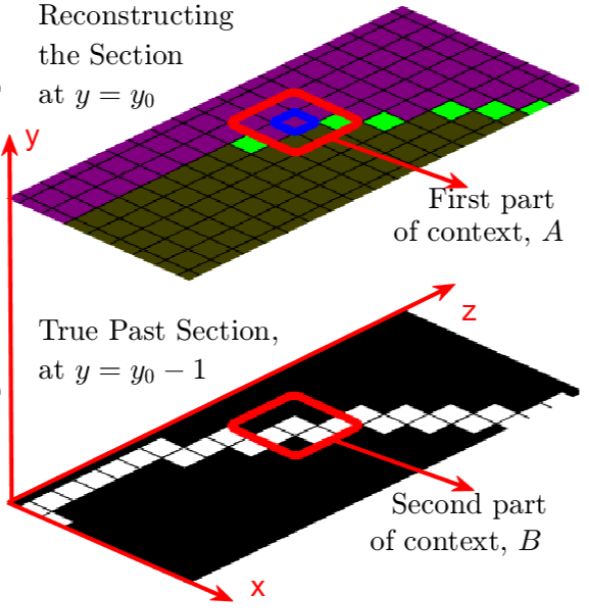
current and the past sections.
2.1. Stage I: Encoding a front and a back depthmap pro-
jection
The first encoding stage is intended for defining and encoding
the maximal and minimal depthmaps (representing heights
above the Oxy plane) resulting in exclusion sets containing
large parts of the space. The minimal depthmap, Zmin , has at
the pixel (x, y) the value, Zmin (x, y) equal to the minimum z
for which (x, y, z) is a point in the original point cloud. Sim-
ilarly, the maximal depthmap, Zmax has at the pixel (x, y)
the value, Zmax (x, y) equal to the maximum z for which
(x, y, z) is a point in the original point cloud. If no point with
(x, y) exists in the point cloud, then it is set Zmin (x, y) =
Zmax (x, y) = 0. The encoding of these depthmaps is per-
formed by CERV [14], which encodes the geodesic lines us-
ing contexts very rich in information.
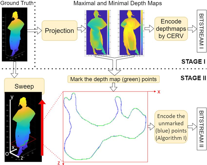
2.2. Stage II: Encoding the remaining points Fig. 1. Overview of the proposed method: In Stage I, minimal
and maximal depthmaps Zmin and Zmax are generated by
At Stage II, we sweep the point cloud along the y dimension, projecting the point cloud along z axis. The depthmaps are
stepping y0 from 0 to Ny −1, and we reconstruct all the points encoded by CERV[14]. In Stage II, the point cloud is swept
in the current section y0 in the (Nz xNx ) binary image R through y axis. The points that are not already encoded by
(current reconstruction). At every y0 , points projected to the CERV (blue points) are encoded as described in Sections 2.2
depthmaps are already known to the decoder and we initialize and 2.3.
the current reconstruction R with the projected points such
that, R(Zmax (x, y0 ), x) = 1 and R(Zmin (x, y0 ), x) = 1 for
every Zmax (x, y0 ) > 0 and Zmin (x, y0 ) > 0. R will be removed from the list, since its occupancy status is already
updated whenever a new point is encoded or decoded. We known. Otherwise, if K(z, x) = 0, we transmit the value
note that, in the binary image R, we know at each column x of T (z, x) using arithmetic coding with the coding distribu-
which are the lowest and the highest occupied points (min- tion stored at the context ζ. After that, the counts of symbols
imal and maximal depths). We consequently construct the associated with the context ζ are updated. K is updated as
binary image F of feasible regions, i.e., of locations in the K(z, x) ← 1 , and the reconstructed image is updated as
plane that are possibly occupied (the magenta pixels in Fig. R(z, x) ← T (z, x). If the value T (z, x) = 1, we include to
2(b)). Formally, F (z, x) = 1 for all (z, x) pair satisfying the list any neighbor (zn , xn ) of (z, x), (in 8-connectivity) for
Zmin (x, y0 ) ≤ z ≤ Zmax (x, y0 ). Using R and F , we initial- which K(zn , xn ) = 0 and for which the marked status is 0,
ize a binary image K, where 1 denotes that the occupancy of a M (zn , xn ) = 0. After inclusion, the marked status is set to 1,
location is known. For example, the locations outside the fea- M (zn , xn ) = 1. This procedure is repeated until the list be-
sible region are known to be unoccupied, hence, K(z, x) = 1 comes empty. At the end, we have encoded all the points that
for those locations. The true points in the section, that we are connected to the boundary of the feasible region by a path
need to losslessly encode, are marked in a binary image de- of connected pixels (in 8-connectivity). After the final section
noted T (see Fig. 2(a)), and the reconstructed points in the y0 = Ny − 1 is processed, all the points that are connected
past section (at y0 − 1, that is already known to the decoder) to the points contained in the initial two depthmap images are
are marked in a binary image P . encoded. For the voxelized point clouds, this outer shell of
In the image R the already reconstructed true points be- points contains the majority of the points in the point cloud.
longing to depthmaps form a set φ of pixels. We perform The remaining points (if any) are encoded by processing ad-
a morphological dilation of the set φ using as structural el- ditional shells, as described in Section 2.4.
ement the 3 × 3 element. This obtained set of locations is
traversed along the rows of the 2D image and is stored in a 2.3. Normalized Contexts
list L. We also initialize a binary marker image M to mark
the pixels already in the list L. After this initialization step, One of the most efficient ways of utilizing the contextual
the list L is processed sequentially, starting from the top of information that is needed in Stage II is described here. In
the list, processing a current pixel (z, x). Both encoder and order to show the elements forming the context, it is illus-
decoder check whether K(z, x) = 1, and if yes, the point is trated in Fig. 2(c) the ground truth occupancies for the cur-Algorithm 1 Stage II of encoding
Require: T : True section binary image at y = y0 (Nz x Nx )
P : True section binary image at y = y0 − 1 (Nz x Nx )
R: Current reconstruction at y = y0 − 1 (Nz x Nx )
F : Feasible Regions bin. image derived from R (Sect. 2.2)
K: Binary image of known locations K ← F + R
L: Pixels to be processed L ← {(z, x) 3 R(z, x) = 1}
M : Binary image of pixels that has been to L. M ← R
(a) (b) while L 6= ∅ do
Read (z, x) from the top of L
Extract a 3x3 matrix R3x3 from R centered at (z, x)
Extract a 3x3 matrix B from P centered at (z, x)
Extract a 3x3 matrix K3x3 by cropping K around (z, x)
A ← R3x3 + K3x3
Find normalizing rotation α∗ (A) and form Aα∗
Use α∗ (A) to rotate B as Bα∗
Form the context ζ = (I(Aα∗ ), J(Bα∗ ))
Encode T (z, x) using the context ζ
if T (z, x) == 1 then
Append to L every neighbor (zn , xn ) of (z, x) for
which K(zn , xn ) = 0 and M (zn , xn ) = 0
(c) (d) If (zn , xn ) is appended, M (zn , xn ) ← 1
end if
Fig. 2. (a) True current section; (b) The feasible region (ma- Update R: R(z, x) ← T (z, x)
genta), points from the depth maps (green), forbidden region Update K: K(z, x) ← 1
(khaki); (c) Details of the ground truth inside the blue rectan- Remove (z, x) from L
gle from (b); (d) Selection of the two part context for encoding end while
the blue marked pixel
sider that we need to encode T (z, x). The first part of the con-
rent section (y = y0 ) and the past section (y = y0 − 1), text uses the values of the already reconstructed pixels that are
showing in white the (true) occupied pixels in these sections. 8-neighbors of (z, x) and also the information about which of
On Fig. 2(d), we show the same area during the reconstruc- the pixels were already known. The values of the pixels in
tion process, which advances section by section such that, at the ternary image Rk = R + K have the following signif-
the moment of reconstructing the section y = y0 , the section icance: Rk (z, x) = 0 if the value of T (z, x) is not known
y = y0 − 1 is fully known, and the second part of the con- yet; Rk (z, x) = 1 if the value of T (z, x) was encoded and
text, called matrix B, can be extracted and contains the true T (z, x) = 0; Rk (z, x) = 2 if the value of T (z, x) was en-
occupancy status at section y = y0 − 1. The context A from coded, and T (z, x) = 1. We consider first the 3×3 square,
the current section for every candidate pixel (z, x) is extracted centered at (z, x), cropped from the image Rk , and we de-
from the 3 × 3 neighbourhood of the pixel (i.e., the pixels in note it as a 3×3 matrix A. The elements of A belong by con-
the red square). struction to 0, 1, 2. The second part of the context is the
When encoding the blue marked pixel, the pixels consid- 3 × 3 binary matrix B formed from P at (z, x). The infor-
ered as the 3×3 A matrix part of context are those surrounded mation from A and B is used to form the context. For ex-
by the red contour. Each pixel might be green (already en- ample scanning by columns weP get a P
one-to-one correspon-
2 2
coded in Stage I), for which the status is known and occu- dence between A and I(A) = j=0 i=0 Aij 3i+3j . Sim-
pied (K(z, x) = 1 and R(z, x) = 1), khaki for forbidden ilarly there
P2is aP one-to-one correspondence between B and
2
pixels with status known and unoccupied (K(z, x) = 1 and J(B) = j=0 i=0 Bij 2i+3j . We combine them to a con-
R(z, x) = 0), and finally magenta for feasible i.e., not yet text label ζ = (I(A), J(B)).
known (K(z, x) = 0). The context extracted from the cur- The context information in A and B is further normal-
rent section forms the matrix A and that from the past section ized in the following way: We consider performing context
forms the matrix B (which are later rotated for normalizing collapsing operations, such that if we would perform a ro-
and are combined to form the final contexts). tation by α ∈ {0, π/2, π, 3π/2} of each of the images R,
The procedure for encoding the points at a section y = y0 T and K around the pixel (z, x), the value of the resulting
with normalized contexts is summarized in Algorithm 1. Con- normalized context is the same. We consider first the 3×3that are connected by a path in 3D space (in 26-voxel con-
Table 1. Average Rate for the first 200 frames from MVUB
nectivity), to the initial points recovered in Stage I from the
[15] and 8i [16] datasets for the proposed Bounding Volume
two depthmap images. However, there are complex point
Lossless (BVL) encoder compared to recent codecs.
clouds, for example those representing a building and objects
inside, where some objects are not connected by a 3D path to
Average Rate [bpv] the outermost points. In that case one can repeat the encod-
Sequence P(PNI)[8] TMC13[9] DD[12] BVL ing process shell by shell, in a peeling-off operation, where
Microsoft Voxelized Upper Bodies [15] we encode first the outermost shell, defined by the points
Andrew9 1.83 1.14 1.12 1.17 represented in the maximal and minimal depthmaps and all
David9 1.77 1.08 1.06 1.10 points connected to these points, and then we reapply the
Phil9 1.88 1.18 1.14 1.20 same process to the remaining un-encoded points. If needed,
Ricardo9 1.79 1.08 1.03 1.05 this peeling-off process can be applied several times. In this
work, there are maximally 2 shells peeled-off and the remain-
Sarah9 1.79 1.07 1.07 1.08
ing points (if any) are simply written in binary representation
Average 1.81 1.11 1.08 1.12
into the bitstream.
8i Voxelized Full Bodies [16]
Longdress 1.75 1.03 0.95 0.91
Loot 1.69 0.97 0.91 0.88 3. EXPERIMENTAL WORK
Redandblack 1.84 1.11 1.03 1.03
Soldier 1.76 1.04 0.96 0.96 The algorithm is implemented in C and the experiments were
Average 1.76 1.04 0.96 0.94 carried out on two point cloud datasets namely, 8i Voxelized
Full Bodies [16] and Microsoft Voxelized Upper Bodies [15].
The average bits per occupied voxel results (average rates)
are presented on Table 1. For each point cloud, all 6 possi-
matrix A. Apply the α rotation around the middle pixel and ble permutations of the 3 dimensions are tried and the best
denote Aα the resulting 3 × 3 matrix. Compute for each rate obtained is kept and reported here. It is observed that,
of α ∈ {0, π/2, π, 3π/2}, the matrix Aα and the weighted proposed method performs better than the other methods on
score of it W (Aα ) and pick as canonical rotation that α∗ for the 8i dataset. On the other hand, on MVUB dataset, our re-
which the weighted score W (Aα ) is the largest. Hence, the sults are slightly worse than TMC13 [9] and Dyadic Decom-
four rotated matrices Aα with α ∈ {0, π/2, π, 3π/2} will position [12]. Additionally, we test BVL and TMC13 on all
be represented only by Aα∗ . This process of collapsing the the point clouds from the Cat1A MPEG Database [17] having
four matrices into a single one is performed offline once, re- original resolutions of 10 and 11 bits. These were quantized
sulting in a tabulated mapping α∗ ↔ A and another map- to 10, 9 and 8 bits as well to test the performance in lower res-
ping I∗ ↔ A, which realize the mappings of the context olutions. BVL outperformed TMC13 in average at 10 bits by
to the canonical one, stored in look-up tables. As an ex- 6.6%, at 9 bits by 5.2%, at 8 bits by 2%. At 11 bits, TMC13
ample of the weighting score W (A), we consider the vector outperformed BVL by 1.8%. For all of the point clouds men-
v = [A00 A01 A10 A02 A11 A20 A12 A21 A22 ] and form W (A) = tioned in this work, the decoding resulted in a perfect lossless
P8 k
k=0 vk 3 , giving in this way a larger weight to those ele- reconstruction.
ments which are close to the corner (0, 0) of A. The normal- Encoding and decoding durations for BVL were measured
ized context is found in the following way: At each point to be 7.3 sec and 7.8 sec, respectively. On the same machine,
(z, x) the matrix A is formed from R+K and the canonical encoding with TMC13 took 1.1 sec. All durations are mea-
rotation index α∗ for this matrix is computed. Also the cor- sured on a single frame of the 10 bits longdress sequence by
responding rotated matrix A0 is computed. The second part running the algorithm 10 times and taking the median. While
of the context is the 3 × 3 matrix B formed from P around the durations are not competitive with TMC13, it should be
(z, x). The matrix B is rotated by the previously determined noted that the execution time is not yet carefully optimized.
α∗ around its center, yielding a matrix B0 . Now the context
to be used for encoding T (z, x) is constructed from A0 and
B0 as context ζ = (I(A0 ), J(B0 )). 4. CONCLUSIONS
2.4. Repetitive peeling-off process for complete recon- We proposed a lossless compression method where the first
struction of more complex point clouds stage is constructing a bounding volume for the point cloud
and the following steps succeed at adding all the remaining
After Stage II, the reconstruction contains all the points form- points at a competitive bitrate, achieving state-of-the-art re-
ing the outer surfaces of the point cloud and all the inner sults for the full body datasets, and comparable results to the
points connected to these outer surface points, i.e., all points current GPCC standard on the upper body dynamic datasets.5. REFERENCES Transactions on Image Processing, vol. 29, pp. 313–
322, 2019.
[1] S. Schwarz, M. Preda, V. Baroncini, M. Budagavi, P. Ce-
sar, P. A. Chou, R. A. Cohen, M. Krivokuća, S. Lasserre, [9] “MPEG Group TMC13,” https://github.com/
Z. Li, et al., “Emerging MPEG standards for point cloud MPEGGroup/mpeg-pcc-tmc13, Accessed: 2020-
compression,” IEEE Journal on Emerging and Selected 03-20.
Topics in Circuits and Systems, vol. 9, no. 1, pp. 133–
[10] D. Meagher, “Geometric modeling using octree encod-
148, 2018.
ing,” Computer graphics and image processing, vol. 19,
[2] L. Cui, R. Mekuria, M. Preda, and Eu. S. Jang, “Point- no. 2, pp. 129–147, 1982.
cloud compression: Moving picture experts group’s new
[11] R. Rosário and E. Peixoto, “Intra-frame compression of
standard in 2020,” IEEE Consumer Electronics Maga-
point cloud geometry using boolean decomposition,” in
zine, vol. 8, no. 4, pp. 17–21, 2019.
2019 IEEE Visual Communications and Image Process-
[3] T. Ebrahimi, S. Foessel, F. Pereira, and P. Schelkens, ing (VCIP). IEEE, 2019, pp. 1–4.
“JPEG Pleno: Toward an efficient representation of vi- [12] E. Peixoto, “Intra-frame compression of point cloud ge-
sual reality,” Ieee Multimedia, vol. 23, no. 4, pp. 14–20, ometry using dyadic decomposition,” IEEE Signal Pro-
2016. cessing Letters, vol. 27, pp. 246–250, 2020.
[4] R. L. De Queiroz and P. A. Chou, “Compression of 3d [13] I. Tabus, E. C. Kaya, and S. Schwarz, “Successive re-
point clouds using a region-adaptive hierarchical trans- finement of bounding volumes for point cloud coding,”
form,” IEEE Transactions on Image Processing, vol. 25, in 2020 IEEE 22nd International Workshop on Multime-
no. 8, pp. 3947–3956, 2016. dia Signal Processing (MMSP). IEEE, 2020, pp. 1–6.
[5] R. Mekuria, K. Blom, and P. Cesar, “Design, implemen- [14] I. Tabus, I. Schiopu, and J. Astola, “Context coding
tation, and evaluation of a point cloud codec for tele- of depth map images under the piecewise-constant im-
immersive video,” IEEE Transactions on Circuits and age model representation,” IEEE Transactions on Image
Systems for Video Technology, vol. 27, no. 4, pp. 828– Processing, vol. 22, no. 11, pp. 4195–4210, 2013.
842, 2016.
[15] C. Loop, Q. Cai, S. O. Escolano, and P. A. Chou,
[6] S. Milani, “Fast point cloud compression via reversible “Microsoft voxelized upper bodies - a voxelized point
cellular automata block transform,” in 2017 IEEE Inter- cloud dataset,” ISO/IEC JTC1/SC29 Joint WG11/WG1
national Conference on Image Processing (ICIP). IEEE, (MPEG/JPEG) input document m38673/M72012, 2016.
2017, pp. 4013–4017.
[16] E. d’Eon, B. Harrison, T. Myers, and P. A. Chou, “8i
[7] Diogo C Garcia and Ricardo L de Queiroz, “Intra-frame voxelized full bodies - a voxelized point cloud dataset,”
context-based octree coding for point-cloud geometry,” ISO/IEC JTC1/SC29 Joint WG11/WG1 (MPEG/JPEG)
in 2018 25th IEEE International Conference on Image input document WG11M40059/WG1M74006, 2017.
Processing (ICIP). IEEE, 2018, pp. 1807–1811.
[17] S. Schwarz, G. Martin-Cocher, D. Flynn, and M. Buda-
[8] D. C. Garcia, T. A. Fonseca, R. U. Ferreira, and R. L. gavi, “Common test conditions for point cloud compres-
de Queiroz, “Geometry coding for dynamic voxelized sion,” Document ISO/IEC JTC1/SC29/WG11 w17766,
point clouds using octrees and multiple contexts,” IEEE Ljubljana, Slovenia, 2018.You can also read