Representation Analysis and Synthesis of Lip Images Using Dimensionality Reduction
←
→
Page content transcription
If your browser does not render page correctly, please read the page content below
International Journal of Computer Vision 67(3), 297–312, 2006

                                                c 2006 Springer Science + Business Media, Inc. Manufactured in The Netherlands.
                                                                                               DOI: 10.1007/s11263-006-5166-3

             Representation Analysis and Synthesis of Lip Images Using
                             Dimensionality Reduction

                               MICHAL AHARON AND RON KIMMEL
 Department of Computer Science, Technion—Israel Institute of Technology, Technion City, Haifa 32000, Israel
                                                michalo@cs.technion.ac.il

                 Received June 11, 2004; Revised February 11, 2005; Accepted August 17, 2005

                                   First online version published in March, 2006

Abstract. Understanding facial expressions in image sequences is an easy task for humans. Some of us are capable
of lipreading by interpreting the motion of the mouth. Automatic lipreading by a computer is a challenging task, with
so far limited success. The inverse problem of synthesizing real looking lip movements is also highly non-trivial.
Today, the technology to automatically generate an image series that imitates natural postures is far from perfect.
   We introduce a new framework for facial image representation, analysis and synthesis, in which we focus just on
the lower half of the face, specifically the mouth. It includes interpretation and classification of facial expressions
and visual speech recognition, as well as a synthesis procedure of facial expressions that yields natural looking
mouth movements.
   Our image analysis and synthesis processes are based on a parametrization of the mouth configuration set of
images. These images are represented as points on a two-dimensional flat manifold that enables us to efficiently
define the pronunciation of each word and thereby analyze or synthesize the motion of the lips. We present some
examples of automatic lips motion synthesis and lipreading, and propose a generalization of our solution to the
problem of lipreading different subjects.

Keywords: automatic lipreading, image sequence processing, speech synthesis, multidimensional scaling, di-
mension reduction, locally linear embedding

1.   Introduction                                                  In this paper we introduce a framework that handles
                                                                frontal view facial images, and is capable of represent-
Automatic understanding and synthesizing of facial              ing, synthesizing, and analyzing sequences of facial
movements during speech is a complex task that has              movements. Our input is a set of frontal facial images.
been intensively investigated (Bregler et al., 1993;            These images are extracted from training sequences of
Vanroose et al., 2002; Li et al., 1997; Bregler et al.,         a single person (the model), that pronounces known
1998; Bregler and Omohundro, 1994; Bregler et al.,              syllables. The ascription of the images to their specific
1997; Kalberer and Van Gool, 2001; Luettin, 1997).              syllable is important, and is used during the synthesis
Improving the technology in this area may be useful             process.
for various applications such as better voice and speech           The images are first automatically aligned with re-
recognition, as well as comprehension of speech in              spect to the location of the nose. Every two images are
the absence of sound, also known as lipreading. At              compared and a symmetric dissimilarity matrix is com-
the other end, generating smooth movements may en-              puted. Next, the images are mapped onto a plane, so
hance the animation abilities in, for example, low bit-         that each image is represented as a point, while trying
rate communication devices such as video conference             to maintain the dissimilarities between images. That is,
transmission over cellular networks.                            the Euclidean distance between each two points on the
298 Aharon and Kimmel
plane should be as close as possible to the dissimilarity Li et al. (1997) investigated the problem of identifi-
between the two corresponding images. We justify this cation of letter’s pronunciation. They handled the first
flat embedding operation by measuring the relatively ten English letters, and considered each of them as a
small error introduced by this process. short word. For training, they used images of a person
Next, the faces representation plane is uniformly saying the letters a few times. All images were aligned
sampled and ‘representative key images’ are chosen. using maximum correlation, and the sequence of im-
Synthesis can now be performed by concatenating the ages of each letter were squeezed or stretched to the
different sequences of images that are responsible for same length. Each such sequence of images was con-
creating the sound, while smoothing the connection verted into a M × N × P column vector, where M × N
between each two sequential sequences. is the size of each image, and P is the number of images
Using the ‘representative key images’, the coordi- in the sequence (simple concatenate of the sequence).
nates of new mouth images can be located on the map. Several such vectors representing the same letter cre-
Each word, which is actually a sequence of mouth im- ated a new matrix, A, of size M N P × S, where S is
ages, can now be considered as a contour, given by the number of sequences. The first eigenvectors of the
an ordered list of its coordinates. Analysis of a new squared matrix A A T were considered as the principle
word is done by comparison of its contour to those of components of the specific letter’s space. Those prin-
already known words, and selecting the closest as the ciple components were called eigen-sequences. When
best match. a new sequence is analyzed, it is aligned as before and
Again, in our experiments, all training sequences and matched with each of the possible letters. First, the new
their corresponding mapping process were done with sequence is squeezed or stretched to the same length
a single subject facial images. Nevertheless, we show of a possible letter’s sequence. Then, the new sequence
that the same concept can be generalized with some is projected onto this letter’s basis, and the amount of
success to lipreading of different subjects, by exploiting preserved energy is tested. The letter which basis pre-
the fact that the sequence of pronounced phonemes in serves most of the new letter energy is chosen as the
the same word is similar for all people. This process re- pronounced letter in the new sequence. In that paper,
quires first correlating between the new person images an accuracy of about 90% was reported.
and the model, and then embedding of the new person’s An interesting trial for lipreading was introduced
pronounced word on the model’s lip configuration sur- by Bregler et al. (1998) under the name of ‘the bar-
face and calculating a new contour. Next, comparison tender problem’. The speaker, as a customer in a bar, is
between the new contour and contours of known words, asked to choose between four different drinks, and due
previously calculated for the model, is computed, and to background noise, the bartender’s decision of the
the closest word is chosen as the analysis result. customer’s request is based only on lipreading. Data
was collected on the segmented lips’ contour, and the
area inside the contour. Then, a Hidden Markov Model
2. Previous Work (HMM) system was trained for each of the four op-
tions. With a test set of 22 utterances, the system was
Automatic understanding (analysis) and generation reported to make only one error (4.5%).
(synthesis) of lip movements may be helpful in various A different approach was used in Mase and Pentland
applications, and these areas are under intense study. (1991), where the lips are tracked using optical flow
We first review some of the recent results in this field. techniques, and features concerning their movements
and motion are extracted. They found that the vertical
lip separation and the mouth elongation capture most
2.1. Analysis of the information about the pronounced word. In the
recognition stage, this information is compared with
The problem of analyzing lip movements, and au- previously known templates, and a decision is taken.
tomatic translation of such movements into mean- Another interesting use in optical flow techniques
ingful words was addressed in several papers. Some for human facial expressions detections was done by
researchers treat lipreading as a stand-alone process Yacoob and Davis (1996). There, the tracking algo-
(Bregler et al., 1998; Li et al., 1997), while others use rithm integrates spatial and temporal information at
it to improve voice recognition systems (Bregler and each frame, and those motion characteristics are used
Omohundro, 1994; Bregler et al., 1993; Luettin, 1997). to interpret human expressions.Representation Analysis and Synthesis of Lip Images 299
The latter techniques extract specific information segmentation of a training audio track, they labelled
about the lips motion and formation, while assum- the facial images, and each sequential three phonemes
ing these features determine most the underlying pro- were handled separately. Next, they segmented the
nounced word (or expression). Here, we preferred to phonemes in the new audio track, and combined triples
work with images of the mouth area, and allow the ap- of phonemes that resembled the segmentation results.
plication decide which are the most dominant features The choice of handling triples of phonemes enabled
that identify the pronunciation. natural connection between all parts of the sentence.
Acoustics-based automatic speech recognition They used a ‘stitching’ process to achieve correspon-
(ASR) is still not completely speaker independent, dence between the synthesized mouth movements and
its vocabulary is limited, and it is sensitive to noise. the existing face and background in the video.
Bregler et al. (1998, 1993) showed, using a neural net- A different synthesis procedure by Bregler et al.
work architecture, that visual information of the lip area (1998) was based on their concept of ‘constrained lip
during speech can significantly improve (up to 50%) the configuration space’. They extracted information on
error rate, especially in a noisy environment. In their the lip contour, and embedded this information in a
experiments, they use a neural network architecture in five-dimensional manifold. Interpolation between dif-
order to learn the pronunciation of letters (each letter ferent images of the mouth was done by forcing the
is considered as a short word). Apart from acoustic interpolated images to lie on this constrained configu-
information, their systems made use of images of the ration space.
lips area (grey level values, first FFT coefficients of Kalberer and Van Gool (2001) and Vanroose et al.
the region around the lips, or data about the segmented (2002) chose to handle 3D faces. They worked with
lip). The results demonstrated that such hybrid systems a system called “ShapeSnatcher”, that uses a struc-
can significantly decrease the error rate. More improve- tured light technique, in order to acquire 3D facial data.
ment was achieved, as expected, when the amount of The 3D structure has an advantage over flat images in
noise was high, or for speakers with more emphasized both analysis and synthesis. It better captures the facial
lips movements, i.e., speakers that move their lips more deformations, it is independent of the head pose, and
while talking. when synthesizing, the geometric information enables
Duchnowski et al. (1995) developed a similar frame- animation of a virtual speaker from several viewing
work for an easy interaction between human and ma- directions.
chine. A person, sitting in front of a computer, was Kalberer and Van Gool (2001) introduced the con-
recorded and videotaped while pronouncing letters. cept of ‘eigenfacemasks’. A 124 vertices in 3D define
The subject’s head and mouth were tracked using a a facial mask, where 38 vertices are located around the
neural network based system. Several types of visual lip area. They acquired face geometry of a single person
features were extracted, such as gray level values, band- pronouncing various phonemes. Each frame was ana-
pass Fourier magnitude coefficients, principal compo- lyzed separately, and represented as a mask. The mask’s
nents of the down sampled image, or linear discrimi- vertices are matched to facial points by marking black
nant analysis coefficients of the down sampled image. dots on the face of the speaking subject. After acquiring
The acoustic and visual data was processed by a multi- several such sequential masks, the first 10 eigenvectors
state time delay neural network system with three lay- were extracted. The space that these eigenvectors span
ers, and 15 units in the hidden layer. By combining the was considered as the space of intra-subject facial de-
audio and visual information, they achieved a 20-50% formations during speech. For animation of a certain
error rate reduction over the acoustic processing alone, word, its viseme1 face masks were displayed, and spline
for various signal/noise conditions. interpolation between the coefficients of the eigenvec-
tors was used to smooth the transitions. The interpola-
tion is between the coefficients of the projection of the
2.2. Synthesis different visemes masks on the chosen eigenvectors.
It means that each intermediate mask was embedded
Bregler et al. (1997) introduced ‘video-rewrite’ as an in the eigenmask space. The eigenfacemasks’ compact
automatic technique for dubbing, i.e. changing a per- space requirements enabled an easy generation of in-
son’s mouth deformations according to a given audio termediate masks, that look realistic.
track. They preferred handling triples of phones, and so In the latter two papers the use of a small lip
achieved natural connection between each two. Using configuration space allows transitions between two300 Aharon and Kimmel
the word, and the syllables that appear before and after
it. One may realize that the main reason for different
pronunciation of the same vowel is the formation of the
mouth just before and after this syllable is said.
In our framework, we divide each word into isolated
parts, each containing a consonant and a vowel, or a
consonant alone, e.g. ‘ba’, ‘ku’, ‘shi’, ‘r’ etc. Each of
these sounds is considered as a syllable. We assume that
each syllable has its own ‘visual articulation signature’
(VAS in short), i.e. the sequence of mouth motions that
Figure 1. Smoothing the transition between different lips configu- must occur in order for the sound to be vocalized. These
rations. mouth motions may differ from one person to another.
Other parts of the full visual pronunciation of a syllable
can be neglected. Figure 2 shows a series of images of
configurations that is restricted to that space. Indeed, a mouth pronouncing the syllable ‘sha’. The VAS is
interpolating on a simple space that captures the lips defined by images 11–19. Here, identification of the
configurations enables efficient natural transitions, and VAS images was done manually.
will be used also in our framework. In Fig. 1, the surface
illustrates a limited 3D lips configuration space, and
3.1. The Input Data
points ‘A’ and ‘B’ are two specific lips configurations
on that manifold. These two configurations are differ-
Our subject (the first author) was videotaped while pro-
ent, so sequential presentation of them might cause
nouncing 20 syllables, each pronounced six times, each
a ‘jerky’ effect. Linear interpolation between the two
time as a different vowel (A, E, I, O, U, and ‘sheva’, a
configurations creates images off the restricted space
consonant that carries an ultra-short vowel or no vowel
(the dashed line), and would look un-natural. A much
sound). Each of the 120 sequences started and ended
better synthesis of a smooth and natural transition be-
with a closed mouth. An example of such a sequence is
tween the two configurations, is restricted to the lips
shown in Fig. 2. For each sequence, the indices of the
configuration space (described as a solid line on the
VAS were registered and recorded. The total number
manifold).
of images was about 3450.
3. Visual Speech Synthesis and Lipreading
by Flat Embedding 3.2. Comparing Images
Different people pronounce the same vowels differ- Alignment: The images were taken using a station-
ently. Even the pronunciation of the same person in ary camera, while the subject was sitting. Nevertheless,
different scenarios may change. We chose to explore slight movements of the head are unavoidable, and the
the case of a single subject speaking to the camera and images were first aligned. As the nose is stable while
slightly accentuating the words. talking, it was chosen as the alignment object. Each
Each vowel is pronounced differently when said in image was translated, using an Affine Motion detec-
different parts of a word. For example, the vowel ‘A’ tor algorithm (Lucas and Kanade, 1981; Bergen et al.,
in ‘America’ looks different from the vowel ‘A’ in ‘Los 1992; Aharon and Kimmel, 2004), so that the nose is
Angeles’. This difference occurs (among other subjec- completely stable. After alignment, only the mouth-
tive reasons) due to the location of the syllable ‘A’ in area (as seen in Fig. 2) was considered.
Figure 2. One syllable image sequence.Representation Analysis and Synthesis of Lip Images 301
1
0.9
0.8
0.7
0.6
0.5
0.4
0.3
Euclidean distance
0.2
L1nor m
0.1 JBB distance
Correlation
0
Figure 3. Comparison between various measures for distance between images.
Comparison Measure: As a distance measure be- all calculated on a slightly smoothed (with a 5 × 5
tween images we chose a variation on the Jacobs, Bel- Gaussian kernel with standard deviation 0.8) version of
humeur, and Basri (JBB) measure (Jacobs et al., 1998), the images. We chose a specific mouth image and com-
given by pared it to 10 randomly selected mouth images, taken
from various pronunciations, at different times, and
I J under slightly different illumination conditions. The
E(I, J ) = I · J ∇ · ∇ d xd y, (1)
J I comparisons results were normalized between 0 (most
similar) and 1 (most different), and are shown in Fig. 3.
where I (x, y) and J (x, y) are two images and E(I, J ) The random images are ordered according to their
is the relative distance between them. JBB distances from the image at the top. The first three
Let us briefly motivate the JBB measure. Assume images describe the same syllable as the top image (al-
that an object {x, y, f (x, y)} is viewed from direction though taken under slightly different illumination con-
( f , f ,1)
(0, 0, −1), its surface normals are √ x2 y 2 . When ditions). Those images were considered closest to the
f x + f y +1
this object, assumed to be Lambertian, is illuminated by original image by both the JBB and the correlation mea-
one light source from direction (s x , s y , s z ), the intensity sure. However, the JBB was able to better enhance the
image is given by difference from images that describe other syllables.
Next, using the JBB measure, we calculated the dif-
−(s x , s y , s z ) · ( f x , f y , 1) ferences between each two images in the input set. We
I (x, y) = α(x, y) , (2)
f x2 + f y2 + 1 thereby obtained an N × N symmetric matrix of rela-
tive distances (dissimilarity measures), where N is the
total number of images.
where α(x, y) is the albedo function of the object.
Dividing two images of the same object, taken un-
der different illumination conditions, the albedos and 3.3. Flattening
the normalization components cancel out one another.
Roughly speaking, the resulting ratio is ‘simpler’ than Our next goal is to embed all the images as points in a
the ratio of two images of different objects. A simple finite dimensional Euclidean space, such that the Eu-
measure of the complexity of the ratio image is the clidean distance between each two images is as close as
integral over its squared gradients |∇( JI )|2 . Symme- possible to the dissimilarity between the images. This
try consideration, and compensating for singularities flat embedding offers a compact representation that
in shadowed areas lead to the above measure. simplifies the recognition process. For our application,
In order to validate the JBB measure, we compared it small distances are more significant than larger ones.
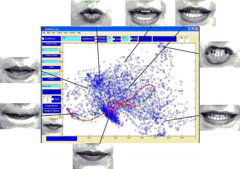
to the L 1 and L 2 norms and to the correlation measure, The reason is that we are interested in representing one302 Aharon and Kimmel Figure 4. The flat embedding onto a plane. image using another that is close to it on the flat sur- part of the screen, while closed mouth images are found face. The accurate distance between two different im- at bottom left. Images that contain teeth are mapped to ages is less important, as long as they are far from each the right, while images without teeth are found at the other on the representation plane. A related flattening left part. procedure was explored by Roweis and Saul (2000) We next investigate three flattening methods - locally with full face images, using locally linear embedding linear embedding, classical scaling and least squares (LLE). multidimensional scaling. Each of these methods was Figure 4 shows the screen of a tool we built in order tested on our data base of images, and their results to explore the properties of the flattening process. The were compared. The chosen embedding space is the embedding flat surface, on which the blue circles are planar mapping shown in Fig. 4. It was found using located, is seen in the middle. Each blue circle repre- least squares MDS with classical scaling initialization. sents an image, where similar looking images are close to each other. The red contour represents a sequence 3.3.1. Locally Linear Embedding. Locally linear of mouth images saying the word ‘Emi’. We see that embedding (Saul and Roweis, 2003) is a flattening this path is divided into two parts, one for each of the method designed for preserving the local structure of two different syllables that define this word. The green the data, and addressing the problem of nonlinear di- stars represent the images that are shown when synthe- mensionality reduction. The mapping is optimized to sizing the word, in order to create a smooth transition preserve the local configurations of nearest neighbors, between the two syllables. The stars lie almost along a while assuming a local linear dependence between straight line, which connects the two parts of the word. them. The ‘neighborhood’ definitions of each point is More about this synthesis procedure a head. set by the user, and may include all points which dis- It is interesting to note that the flattening procedure tances from a given point is smaller than a certain value, we use maps the open mouth images to the upper right a fixed number of closest points, or any other reasonable
Representation Analysis and Synthesis of Lip Images                303

neighborhood definition. Given an input set of N data         sumes that the dissimilarities between the images are
points X 1 , X 2 , . . . X N , the embedding procedure is     Euclidean distances in some d-dimensional space.
divided into three parts:                                     Based on this assumption it reveals a centered configu-
                                                              ration of points in a d-dimensional world, that best pre-
– Identify the neighbors of each data point, X i .            serves, under Frobenius norm, those distances. Classi-
– Compute the weights Wi j that best reconstruct each         cal scaling’s solution in a d-dimensions minimizes the
  data points X i from its neighbors, by minimizing           following function,
  the cost function

                                           2                   B − τ1 (2 )2 ,     subject to           B ∈ n (d),    (5)


                                                                                F
            E(W ) =     Xi −      Wi j X j  .    (3)
                      i
                                j
                                                             where n (d) is the set of symmetric n × n positive
                                                              semi-definite matrices that have rank no greater than
  A least squares problem.                                    d, 2 = [δi2j ] is the matrix of squared dissimilarities,
– Compute the embedded points Yi in the lower di-             τ1 (D) = − 12 (I − 11 )D(I − 11 ) is the double cen-
  mensional space. These coordinates are best recon-          tering operator, and 1 = [1, . . . , 1] ∈ R n .
  structed (given the weights Wi j ) by minimizing the           This method includes four simple steps. Let 2 be
  equation                                                    the matrix of squared dissimilarities.
                                        2

                                                             – Apply double centering: B = τ1 (2 ).
             (Y ) =    Yi −   Wi j Y j  .         (4)      – Compute eigendecomposition of B = QQ  .
                     i
                             j

                                                              – Sort the eigenvalues, and denote
   An eigenvalue problem.
                                                                                     ii   if ii > 0, i < d
                                                                           ii+ =
   The output of the algorithm is a set of points{Yi }i=1
                                                      N                              0     otherwise
in a low dimensional space, that preserves the local
                                                              – Extract the centered coordinates by X = Q+
                                                                                                                          1/2
structure of the data. A more detailed description of                                                                           .
this method is given in Aharon and Kimmel (2004).
   In our case, the input to the LLE algorithm was the           If the distances would have been indeed between
matrix of pairwise distances between each two points,         points in a d-dimensional Euclidean space, then clas-
and not the initial coordinates of each point (which          sical scaling provides the exact solution. Otherwise, it
would have been the image gray-level values). We              provides only an approximation, and not necessarily
therefore derived from this matrix the neighborhood           the one we would have liked.
relations and the weights calculations, as described in          In our application, we tested the classical scaling
(Saul and Roweis, 2003; Aharon and Kimmel, 2004).             solution in two-dimensional space. The coordinates in
   An improvement to the LLE algorithm and the re-            the representation planar space are given by the first
lated Isomap (Tenenbaum et al., 2000) was proposed            two eigenvectors of the double centered distances ma-
by Donoho and Grimes (2003) by the name of ‘Hessian           trix, scaled by their corresponding (largest) eigenval-
Eigenmaps’. That method can handle the case of a con-         ues. This method also provides the accuracy of the rep-
nected non-convex parametrization space. We did not           resentation captured by the first two eigenvalues, which
experiment with this method.                                  can be measured by the following ‘energy’ term, (a
                                                              variation of the Frobenius norm)
3.3.2. Classsical Scaling. Multidimensional scaling
(MDS) (Borg and Groenen, 1997), is a family of meth-                                        2
                                                                                                  λi2
ods that try to represent similarity measurements be-                            E=         i=1
                                                                                            N
                                                                                                        ,                  (6)
tween pairs of objects, as distances between points in a                                    i=1   λi2
low-dimensional space. This allows us to visually cap-
ture the geometric structure of the data, and perform         where λi is the ith largest eigenvalue of the distances
dimensionality reduction.                                     matrix, after double centering. In our case, the first
   First we tested classical Scaling (Borg and Groenen,       two eigenvalues capture approximately 95% of the en-
1997; Aharon and Kimmel, 2004). This method as-               ergy. This number validates the fact that our images
304 Aharon and Kimmel
can be embedded in a plane with insignificant distor- Table 1. Stress values for different variations of MDS. The
tion, which is somewhat surprising. weighted stress is calculated with wi j = 1/δi2j .
Un-weighted Weighted
3.3.3. Stress Definitions. Classical scaling prefers Method stress stress
the order by which the axes are selected, and thus min-
Classical MDS 0.095 0.1530
imize the Frobenius norm. Next, we use an unbiased
measure, that takes into consideration the dimension Least Squares MDS with 0.159 0.0513
random initialization
of the target space, in order to evaluate the quality of
Least Squares MDS with 0.022 0.0550
the flattening procedure (Borg and Groenen, 1997). We
LLE initialization
first define the representation error as
Least Squares MDS with Classical 0.022 0.0361
Scaling initialization
ei2j = (δi j − di j )2 , (7)
where δi j and di j are the dissimilarity and the Euclidean Table 2. Stress values for different versions of LLE. The
distance in the new flat space between points i and j, weighted stress is calculated with wi j = 1/δi2j .
respectively. The total configuration’s representation Un-weighted Weighted
error is measured as the sum of ei2j over all i and j, that Method stress stress
defines the stress
Fixed number of neighbors (5) 0.951 0.948
σ (X ) = (δi j − di j )2 . (8) Fixed number of neighbors (20) 0.933 0.948
i< j Fixed Threshold (0.019) 0.927 0.930
Here di j is the Euclidean distance between points i
and j in the configuration X . In order to weigh dif-
ferently smaller and larger distances, we consider a stress values were worse than the one achieved by clas-
weighted sum sical scaling. We thus initialized the algorithm with a
configuration that was found by classical scaling. That
σW (X ) = wi j (δi j − di j )2 . (9) yielded a significant improvement (see Table 1). We
i< j also tried to multiply the classical scaling configura-
tion by a scalar according to the suggestion of Malone
Finally, we normalize the stress to obtain a com- et al. (2000) for a better initial configuration for the
parable measure for various configurations with some least squares procedure. In our experiments this initial-
insensitivity to the number of samples, ization did not improve the final results.
We search for a configuration that better preserves
i< j wi j (δi j − di j )2 small distances, and gives higher accuracy. For that
σ̂W (X ) = . (10)
wi j · δi2j end, we defined a weight matrix, that is derived from
i< j
the dissimilarities matrix by wi j = 1/δi j , In this
Using this measure, we can compare between vari- case, errors are defined by the relative deformation. By
ous flattening methods. The stress results for classical this normalization, larger distances can suffer larger
scaling and LLE, calculated without weights, and with deformations.
weights wi j = 1/δi2j , are given in Tables 1 and 2.
3.3.5. Flattening Methods—Comparison. All the
3.3.4. Least Squares Multidimensional Scaling. three methods were applied to our data base. The stress
Least-Square MDS (Borg and Groenen, 1997) is a values (weighted and un-weighted) of classical scaling
flattening method that directly minimizes the stress and least squares MDS (with different initial configura-
value in Eq. (10). The optimization method we used is tions) can be seen in Table 1. Stress values are computed
called iterative majorization (Borg and Groenen, 1997; with the same weights used in the minimization.
Aharon and Kimmel, 2004). The initial configuration We also tested LLE using three different neighbor-
of the least squares MDS is crucial, due to the exis- hood definitions: 5 nearest neighbors for each point,
tence of many local minima. In our experiments, when 20 nearest neighbors for each point and all neighbors
initialized with a random configuration, the resulting which distances to the point is less than 0.019 (betweenRepresentation Analysis and Synthesis of Lip Images 305
1 and 1102 neighbors for each point). The results were 2. The JBB distances between the new image, and each
tested by calculating the un-weighted stress value, and of the ‘representative key images’ were calculated.
the weighted stress value with the same weights as 3. The coordinates of the new image are set as a
before (wi j = 1/δi2j ). The results are presented in weighted sum of the representatives’ coordinates,
Table 2. according to the distance from each representative.
Another recent method for dimensionality reduction,
which we did not investigate, is the ‘Isometric feature N
i=1 wi · x i
mapping’ or ISOMAP (Tenenbaum et al., 2000), see xnew = N
, (11)
Schwartz et al. (1989) for an earlier version of the i=1 wi
same procedure. This method assumes that the small
measured distances approximate well the geodesic dis- where N is the number of ‘representative key im-
tances of the configuration manifold. Next, using those ages’, xi is the x coordinate of the ith representative
values, geodesic distances between faraway points are key image and the weight wi is set to be 1/δi3 , where
calculated by a graph search procedure. Finally, classi- δi is the JBB distance between the new image, and
cal scaling is used to flatten the points to a space of the the ith representative key image. The y coordinate
required dimension. Isomap introduces a free param- was calculated in a similar way.
eter that sets the neighborhood size, and prevents us
from comparing reliably between the various methods.
3.5. Sentence Synthesis
In our application, using Least-Squares MDS enabled
us to decrease the influence of large distances. Weight-
A simple way to synthesize sequences using the facial
ing the importance of the flattened distances can replace
images is by concatenating the VAS of the syllables
the need to approximate large distances, as is done to in
that integrate into the sentence, so that the ‘crucial’
Isomap.2 Moreover, we demonstrate empirically, that
part of each syllable is seen. The first and last part of
the small stress values computed by the flat embed-
the sequence of pronunciation of each syllable appears
ding via Least-Squares MDS validates the numerical
only if this syllable is at the beginning or the end of the
correctness of the method we used for the lips images.
synthesized word, respectively.
This concatenating procedure results in unnatural
3.4. Space Parametrization speaking image sequences because the connection be-
tween the different partial sequences is not smooth
Thousands of images were flattened to a plane, and enough. An example can be seen in Fig. 5. There, a
generated regions with varying density, as can be seen simple synthesis of the name “Emi” is performed as
in Fig. 4. In order to locate the coordinates of a new described above, and the transition between the two
image in the plane, we first select ‘representative key syllables (images 14 and 15) can be easily detected.
images’ by uniformly sampling the plane. We use only
this sub-set of images to estimate the coordinates of a
new image. In our experiments we selected 81 images
(out of 3450) to sample the representation plane. This
was done by dividing the plane into 100 squares (10
squares in each row and column). For each square that
contained images, the image which is closest to the
median coordinates was selected as a ‘representative
key image’ (the median coordinate in both x and y
were calculated, and then the image which is closest
to this point was selected). Next, in order to locate the
coordinates of a new image in the representation plane
the following steps were followed.
1. The nose in the new image is aligned, by comparing
to one of the previously taken images, using an affine
motion tracker algorithm. Figure 5. Simple synthesis sequence of the name “Emi.”306 Aharon and Kimmel Figure 6. Smooth transition between images 14 and 15 in Fig. 5. A possible solution to this problem is by defining images may slow down the pronunciation, whereas the a weighted graph clique; a graph in which there is a duration of the pronunciation and synchronization with weighted edge between each two vertices. The vertices the sound is crucial when synthesizing speech. We, represent the input images and the weight of the edge therefore, control the number of images that are dis- between vertex i and j is the dissimilarity measure be- played by re-sampling the sequence. An example of a tween the two corresponding images. A smooth tran- shorter smooth transition is shown in Fig. 7. sition between images A and B can be performed by Another solution, that exploits the embedding sur- presenting the images along the shortest path between face and the chosen representative key images is to A and B. This path is easily found using Dijkstra’s define a clique weighted graph which nodes are the algorithm. The shortest path between an image at the representative key images, and the two images between end of the VAS of the first syllable, and an image at the which the smoothing should be done. The weight of the beginning of the VAS of the next syllable is used to syn- edge that connects images i and j is the distance mea- thesis smooth transactions, as shown in Fig. 6. There, sure between the two images. The smooth transition 16 images, marked as ‘new’, were found by the Dijk- contains the images along the shortest path between the stra algorithm as the shortest weighted path between two images. Computing this solution is much faster, as the last image of the viseme signature of the phoneme the Dijkstra algorithm runs on a much smaller graph. ‘E’ (number 14) and the first image of the viseme sig- The paths that are found rarely need re-sampling, as nature of the phoneme ‘Mi’ (number 15). This smooth they are much shorter than those in the full graph. An connection between two different lips configurations is example of the synthesis of the name ’Emi’ appears in obviously embedded in the constrained lips configura- Fig. 8. tion space. The synthesis procedure is completely automatic. In this solution, a problem may occur if the path The input is defined by the text to be synthe- that is found includes too many images. Merging those sized and possibly the time interval of each syllable Figure 7. Sampled transition between images 14 and 15 in Fig. 5. Figure 8. Smooth transition between images 14 and 15 in Fig. 5, using the (sampled) embedding-based synthesis method.
Representation Analysis and Synthesis of Lip Images                    307

pronunciation, as well as the pauses between the words.             indices of the minimum chosen values (each index can
The results look natural as they all consist of realistic,          vary from 1 to 3, for the 3 possible values of g(i, j))
aligned images, smoothly connected to each other.                   indicates the new parametrization of the sequence A,
                                                                    in order to align it with the parametrization of the se-
                                                                    quence B. Using dynamic programming, the maximum
3.6.   Lipreading
                                                                    number of Euclidean distance computations is m · n,
                                                                    and therefore, the computation is efficient.
Here we extend the ‘bartender problem’ proposed by
                                                                       When a new parametrization s is available, the first
Bregler et al. (1998). We chose sixteen different names
                                                                    derivative of sequence A is calculated using backward
of common drinks,3 and videotaped a single subject
                                                                    approximation x s A = xsA −xs−1A
                                                                                                      , and second derivatives
(the same person that pronounced the syllables in the                                           A
                                                                    using a central scheme x s = xs+1    A
                                                                                                            − 2xsA + xs−1
                                                                                                                        A
                                                                                                                           . In
training phase) saying each word six times. The first
                                                                    this new parametrization the number of elements in
utterance of each word pronunciation was chosen as
                                                                    each sequence is the same, as well as the number of
reference, and the other utterances were analyzed, and
                                                                    elements of the first and second derivatives, that can
compared to all the other reference sequences. After
                                                                    now be easily compared. Next, three different distance
the surface’s coordinates of each image in each word
                                                                    measures between the two contours are computed
sequence (training and test cases) are found, each word
can be represented as a contour. Analyzing a new word
reduces to comparing between two such contours on                    G(A, B) = g(m, n)
                                                                               n           2        2
the flattened representation plane.                                                    A  B      A B
                                                                     P(A, B) =       x s −x s + ys −ys
                                                                                  s=1
Comparing Contours: The words’ contours, as an
                                                                                 n
                                                                                                          2                    2
ordered list of coordinates, usually include a different             Q(A, B) =           x  s − x  s
                                                                                            A          B
                                                                                                                + y  s − y  s
                                                                                                                       A        B
                                                                                                                                       .
number of images. In order to compare two sequences                               s=1
we first fit their lengths. We do so by using a version                                                                             (13)
of the Dynamic Time Warping Algorithm (DTW) of
Sakoe and Chiba (1978) with a slope constraint of one.              Those measures are used to identify the closest refer-
This algorithm is commonly used in the field of speech              ence word to a new pronounced word.
recognition (Li et al., 1997). The main idea behind the                Let us summarize the whole analysis process. When
DTW algorithm is that different utterances of the same              receiving a new image sequence N ,
word are rarely performed at the same rate across the
entire utterance. Therefore, when comparing different
                                                                    1. find the path that corresponds to the sequence by lo-
utterances of the same word, the speaking rate and the
                                                                       cating the representation plane coordinates of each
duration of the utterance should not contribute to the
                                                                       image in the sequence as described in Section 3.4.
dissimilarity measurement.
                                                                    2. For each reference sequence R j , for j = 1 to k,
   Let us denote the two sequences images as: A =
                                                                       where k is the number of reference sequences (16
[a1 , a2 , . . . am ], and B = [b1 , b2 , . . . bn ], where ai =
                                                                       in our experiments) do:
{xi , yi } are the x and y coordinates of the i − th image
in the sequence. We first set the difference between
                                                                       (a) Compute the DTW between the sequence N and
images a1 and b1 as g(1, 1) = 2d(1, 1), where d(i, j)
                                                                           Rj.
is the Euclidean distance ai − b j 2 . Then, recursively
                                                                       (b) Use these results to compute the distances
define
                                                                           G(N , R j ), P(N , R j ), and Q(N , R j ).
g(i, j)
      ⎧                                          ⎫                  3. Normalize each distance by
      ⎨g(i − 1, j − 2) + 2d(i, j − 1) + d(i, j), ⎬
 = min g(i − 1, j − 1) + 2d(i, j),                 .
      ⎩                                          ⎭
                                                                                                                 k
        g(i − 2, j − 1) + 2d(i − 1, j) + d(i, j)                            G̃(N , R j ) = G(N , R j )                 G(N , Ri )
                                                (12)                                                             i=1


                                                                                                                 k
Where g(i, j) = ∞, if i or j is smaller than 1. The                         P̃(N , R j ) = P(N , R j )                 P(N , Ri )
distance between sequences A and B is g(m, n). The                                                               i=1
308 Aharon and Kimmel
16
14
12
10
Classified Words
8
Euclidean distance
First derivative
Second derivative
6 Combined distance
4
2
0
1 2 3 4 5 6 7 8 9 10 11 12 13 14 15 16
Tested Words
Figure 9. Analysis results of the different distance measures.
k errors). A careful inspection of the misclassified words,
Q̃(N , R j ) = Q(N , R j ) Q(N , Ri ). we noticed that those were pronounced differently be-
i=1 cause of a smile of other spasm in the face. When ana-
(14)
lyzing single words, those unpredictable small changes
4. For each reference sequence, compute the distances are hard to ignore. The results of the different measures
(Euclidean, first, second derivatives, and their combi-
D j (N ) = G̃(N , R j ) + α · P̃(N , R j ) nation) can be viewed in Fig. 9. The 96 utterances are
divided into 16 groups along the x axis. The diamond,
+ β · Q̃(N , R j ). (15) circle, and star icons indicate the analysis results com-
puted with the Euclidean, first derivative, and second
In our experiments, we empirically found that α =
derivative distance, respectively. The line indicates the
β = 12 give the best classification results.
result of the approximated Sobolev norm that com-
5. Select the closest reference sequence, the one with
bines the three measures. The six miss-classifications
the smallest distance D j (N ), as the analysis result.
are easily detected as the deviations from the staircase
structure. We see that the Euclidean distance is more
The combination of the integral Euclidean distance
accurate than the noisy first and second derivative dis-
with the first and second derivatives is an approxima-
tances. That was the reason for its relative high weight
tion of the Sobolev Spaces norm, defined as
in the hybrid Sobolev norm. The combination of the
k three measures yield the best results.
f 2H 2 = f ( j) 2 2 = f 2 + f 2 + f 2 . We believe that an increase of the number of differ-
L
j=0 ent identified words will be difficult using the above
(16)
framework, mainly due to the current small differences
between each two words. Which is an indication that
We next show that this hybrid norm gives better clas-
lip-reading is intrinsically difficult. However, support-
sification results than each of its components alone.
ing an ASR system, differing between 2–3 possible
Results: We tested 96 sequences (16 words, 6 utter- words or syllables is often needed in order to achieve
ances of each word, one of which was selected as the higher identification rates. In this case, our framework
reference sequence). The accuracy rate is 94% (only 6 would be useful.Representation Analysis and Synthesis of Lip Images 309
Figure 10. Pronunciation of two different people.
3.7. Generalization: Lipreading Other People located on the representation plane using the method
described in Section 3.4. The new person’s visemes
Up until now, we handled facial images of a single are assigned exactly the same coordinates. In our ex-
person (female). Here, we present a generalization in periments, the process of assigning an image for each
which we lip read other people. Instead of performing phoneme was done manually. Figure 11 shows part of
the whole learning process, we exploit the fact that the visemes we assigned for the model and the new
different people say the different words in a similar way. person.
That is, the sequence of pronounced phonemes is equal, Next, the location of the new person’s images on the
when saying the same word. Therefore, after a proper surface is found using the following procedure.
matching between the lips configuration images of the
model and the new person, we expect the representing – The image is compared to all the assigned visemes
contours of the same word to look similar. of the same person, resulting the similarity measures
For that end, we took pictures of second person {δi }i=1
N
, where N is the number of visemes.
(male), pronouncing the various drinks’ names, three – The new coordinates of the image is set by
times each word. In Fig. 10 we can see the two people
N
pronouncing the word ‘Coffee’. i=1 wi · x i
xnew = , (17)
Comparing mouth area images of two different peo- N
i=1 wi
ple might be deceptive because of different facial fea-
tures such as the lips thickness, skin texture or teeth where xi is the x coordinate of the ith viseme and
structure. Moreover, different people pronounce the the weight wi is set to be wi = 1/δi2 . The y coordi-
same phonemes differently, and gray level or mouth’s nate is set in a similar way.
contour comparison between the images might not re-
veal the true similarity between phonemes. For that In the above procedure, only images of the same per-
end, we aligned the new person’s nose to the nose of son are compared. This way, each new person’s image
the model using Euclidean version of Kanade-Lucas. can be located on the representation plane, and each
An affine transformation here may cause distortion of new pronounced word is described as a contour which
the face due to different nose structures. Next, the rest can be compared with all the other contours. In Fig. 12
of the images are aligned to the first image (of the same four such contours are shown, representing the pronun-
person) using affine Kanade-Lucas algorithm, so that ciation of the words ‘Cappuccino’ and ‘Sprite’ by two
all the mouth area images can be extracted easily. different people – the model on the left, and the second
Then, we relate between images of the new per- person on the right.
son and our model by defining a set of phonemes, For comparison between pronunciation contours of
and assigning each phoneme a representing image two different people we added two additional measures,
(also known as viseme). The visemes of the model are which we found helpful for this task,310 Aharon and Kimmel
Figure 11. Visemes assignment. Partial group of the visemes we assigned for the model (left) and the new person.
– maximum distance, which is defined by
min {d(X sA − X sB )} (18)
1≤s≤n
where X sA = [xsA , yxA ] and X sB = [xsB , yxB ] are the
parametrization of the two contours, as seen in Sec-
tion 3.6, after executing DWT, and d(X, Y ) is the
Euclidean distance between points X and Y .
– Integrated distance, defined by
d(X sA − X sB ). (19)
1≤s≤n
Figure 12. Contours representation of words pronunciation.
The above two measures refer only to the
parametrization of the contour after processing DWT.
The maximum distance measures the maximum dis- identification. This conclusion is based on the fact that
tance between two correlated points on the two con- the lowest identification rate were for names composed
tours, and the integrated distance accumulates the Eu- of two words (‘Bloody Mary’,‘Milk Shake’,‘Orange
clidean distances between the correlated points. Juice’ and ‘French Vanilla’). There especially, although
We discovered that the derivative distances that were pronouncing all the phonemes in the same order, dif-
defined in 3.6 and helped comparing between two con- ferent people connect differently between the words.
tours of the same person, were too noisy in this case. Considering only the single word-drinks a success rate
The inner structure (first and second derivatives) of the of 69% is achieved, and considering the first two an-
contour was less important than its coordinates. An ex- swers, we reach 80% success rate.
ample can be seen in Fig. 12 where contours of the
same pronounced word are shown. The point locations
of the two contours is similar, but their inner structure 3.8. Choosing Drink Names in Noisy Bars
is different.
The identification rate was 44% in the first trial, and Next, we explore the following question, ‘What kind
reached 60% when allowing the first two answers (out of drink names should be chosen in a noisy bar, so that
of 16) to be considered. We relate this relatively low a lipreading bartender could easily recognize between
success rate to the assumption that different people pro- them?’. To answer this question, we measured the dis-
nounce the transitions between phonemes differently, tances between each two contours from the set of 96
and therefore, correlating between the phoneme’s im- calculated drink sequences. We received a distances
ages of two different people is not enough for perfect matrix, and performed Classical Scaling. The first twoRepresentation Analysis and Synthesis of Lip Images 311
15
16
10
8
16 8 8
3 16 8
16 8
16 9
15 8 9
5 3 16 12
3 14 12
3 15 14 14 9
7 15 14
14
7 3 15 15
15 9 12 9
7 14 9 12
7 13 12 12
13
13
0 1 13
7 13 11
7 5 1 11 11
5 1
5 1 10 11 11
5 5 11
5 1 1 22
22 10 10
2 4
−5 4 44 10
3 2 10 10
44
−10
6 6
6 6
6 6
−15
−15 −10 −5 0 5 10 15
Figure 13. Choosing drink names in noisy bars.
eigenvectors captured 88% of the energy, and the first The embedding surface is then used to represent each
three 92%. The map presented in Fig. 13, shows that pronounced word as a planar contour. That is, a word
the drinks: ‘Bacardi’ (1), ‘Martini’ (5), ‘Champagne’ becomes a planar contour tracing the points on the
(6), ‘Milk Shape’ (8),‘Vodka’ (10), ‘Cappuccino’ (11) plane for which each point represents an image. The lip
and ‘liqueur’ (14) have more distinct names. Putting reading (analysis) process was thereby reduced to com-
them on the menu, possibly with ‘Cola’ (4) (but with- paring between planar contours. Comparison between
out ‘Coffee’ (2)), or ‘Orange Juice’ (9) (but without words was then done using an efficient dynamic pro-
‘French Vanilla’ (12)), would ease lipreading of the gramming algorithm, based on Sobolev spaces norms.
customers requests. Finely, generalization of the lipreading process was
performed with promising results by exploiting the fact
that the sequence of pronounced phonemes is similar
to all people pronouncing the same word. This was
4. Summary done by first correlating between a given model and
and new subject lips configurations, and then compar-
We introduced a lipreading and lips motion synthesis ing images of the same person only. This way, we find
framework. We qualitatively justified and used the JBB a warp between the representation planes of two un-
measure for distance evaluation between different im- related subjects. We then recognize words said by the
ages, a measure that is robust to slight pose changes new subject by matching their contours to known word
and varying illumination conditions. contours of our model.
We then flattened the visual data on a representation Our experiments suggest that exploring the geomet-
plane. A process we referred to as flattening. This map, ric structure of the space of mouth images, and the
which captures the geometric structure of the data, en- contours plotted by words on this structure may pro-
abled us to sample the space of lips configurations by vide a powerful tool for lip-reading. More generally,
uniformly selecting points from the embedding surface we show that dimensionality reduction for images can
(the representation plane). Using those selected repre- provide an efficient tool for representation of a single
sentatives and the Dijkstra algorithm, we managed to image or a sequence of images from the same family.
smoothly tile between two different images, and syn- It can therefor offer a way to perform synthesis and
thesize words. analysis for such sequences.312 Aharon and Kimmel
Acknowledgments Proceedings of the National Academy of Arts and Sciences,
100(10):5591–5596.
This research was partly supported by European FP 6 Duchnowski, P., Hunke, M., Bsching, D., Meier, U., and Waibel,
A. 1995. Toward movement-invariant automatic lipreading and
NoE grant No. 507752 (MUSCLE). speech recognition. In Proc. ICASSP’95, pp. 109–112.
Fisher, C.G. 1968. Confusions among visually perceived consonants.
Journal of Speech and Hearing Research, 11(4):796–804.
Notes Jacobs, D.W., Belhumeur, P.N., and Basri, R. 1998. Comparing
images under variable illumination. In Proc. of CVPR, pp. 610–
1. The term ‘viseme’ (Fisher, 1968) is a compound of the words 617.
‘visual’ and ‘phoneme’, and here represents the series of visual Kalberer, G.A. and Van Gool, L. 2001. Lip animation based on
face deformations that occur during pronunciation of a certain observed 3d speech dynamics. In Proc. of SPIE, S. El-Hakim and
phoneme. A. Gruen, editors, vol. 4309, pp. 16–25.
2. Note that evaluating distance by graph search introduces metri- Li, N., Dettmer, S., and Shah, M. 1997. Visually recognizing speech
cation errors and the distances would never converge to the true using eigensequences. In Motion-Based Recognition. Klwer Aca-
geodesic distances. This argument is true especially when the demic Publishing, pp. 345–371.
data is sampled in a regular way, which is often the case. Lucas, B.D. and Kanade, T. 1981. An iterative image registration
3. The tested drink names: Bacardi, Coffee, Tequila, Cola, Martini, technique with an application to stereo vision. In IJCAI81, pp.
Champagne, Bloody Mary, Milk Shake, Orange Juice, Vodka, 674–679.
Cappuccino, French Vanilla, Lemonade, Liqueur, Sprite, Sun- Luettin, J. 1997. Visual Speech And Speaker Recognition. PhD thesis,
rise. University of Sheffield.
Mase, A. and Pentland, K. 1991. Automatic lipreading by optical
flow analysis. Technical Report Technical Report 117, MIT—
References Media Lab.
Malone, S.W., Tarazaga, P., and Trosset, M.W. 2000. Optimal dila-
Aharon, M. and Kimmel, R. 2004. Representation analysis and syn- tions for metric multidimensional scaling. In Proceedings of the
thesis of lip images using dimensionality reduction. Technical Statistical Computing Section.
Report CIS-2004-01, Technion—Israel Institute of Technology. Roweis, S.T. and Saul, L.K. 2000. Nonlinear dimensionality reduc-
Bergen, J.R., Burt, P.J., Hingorani, R., and Peleg, S. 1992. A three- tion by locally linear embedding. Science, 290:2323–2326.
frame algorithm for estimating two component image motion. Sakoe, H. and Chiba, S. 1978. Dynamic programming algorithm
IEEE Trans on PAMI, 14(9). optimization for spoken word recognition. IEEE Trans. ASSP,
Bregler, C., Covell, M., and Slaney, M. 1997. Video rewrite: Driving ASSP-26:43–49.
visual speech with audio. Computer Graphics, 31:353–360. Saul, L.K. and Roweis, S.T. 2003. Think globally, fit locally: Un-
Borg, I. and Groenen, P. 1997. Modern Multidimensional Scaling— supervised learning of low dimensional manifolds. Journal of
Theory and Applications. Springer-Verlag New York, Inc. Machine Learning Research, pp. 119–155.
Bregler, C., Hild, H., Manke, S., and Waibel, A. 1993. Improving Schwartz, E.L., Shaw, A., and Wolfson, E. 1989. A numerical solu-
connected letter recognition by lipreading. In Proc. IEEE Int. tion to the generalized mapmaker’s problem: Flattening non con-
Conf. on ASSP, pp. 557–560. vex polyhedral surfaces. 11(9):1005–1008.
Bregler, C. and Omohundro, S.M. 1994. Surface learning with ap- Tenenbaum, J.B., de Silva, V., and Langford, J.C. 2000. A global ge-
plications to lipreading. In NIPS, vol. 6, pp. 43–50. ometric frame-work for nonlinear dimensionality reduction. Sci-
Bregler, C., Omohundro, S.M., Covell, M., Slaney, M., Ahmad, S., ence, 290:2319–2323.
Forsyth, D.A., and Feldman, J.A. 1998. Probabilistic models of Vanroose, P., Kalberer, G.A., Wambacq, P., and Van Gool, L. 2002.
verbal and body gestures. In Computer Vision in Man-Machine In- From speech to 3D face animation. Procs. of BSIT.
terfaces, R. Cipolla and A. Pentland (eds), Cambridge University Yacoob, Y. and Davis, L.S. 1996. Recognizing human facial ex-
Press. pressions from long image sequences using optical flow. IEEE
Donoho, D.L. and Grimes, C.E. 2003. Hessian eigenmaps: new Transactions on Pattern Analysis and Machine Intelligence,
locally linear embedding techniques for high-dimensional data. 18(6).You can also read