Resonance In the Solar System
←
→
Page content transcription
If your browser does not render page correctly, please read the page content below
Resonance In the Solar
       System
              Steve Bache

               UNC Wilmington
  Dept. of Physics and Physical Oceanography
           Advisor : Dr. Russ Herman

               Spring 2012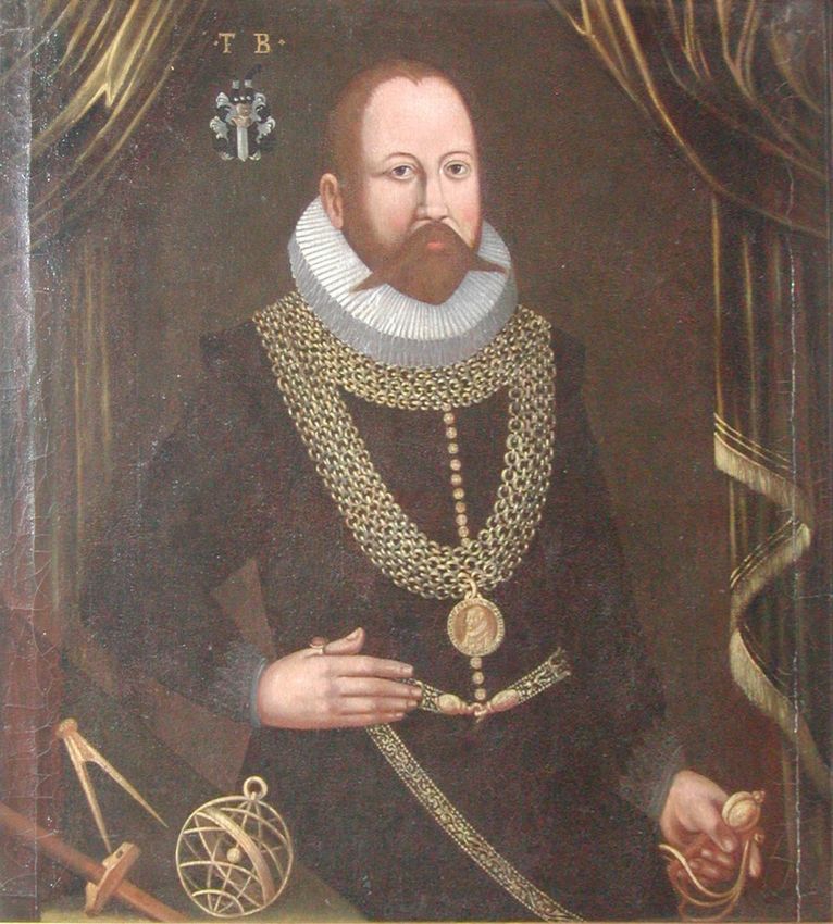
Goal

  • numerically investigate the dynamics of the asteroid belt
  • relate old ideas to new methods
  • reproduce known results
History

 The role of science:
   • make sense of the world
   • perceive order out of apparent randomness
History

 The role of science:
   • make sense of the world
   • perceive order out of apparent randomness
   • the sky and heavenly bodies
Anaximander (611-547 BC)
  • Greek philosopher, scientist
  • stars, moon, sun 1:2:3

                   Figure: Anaximander’s Model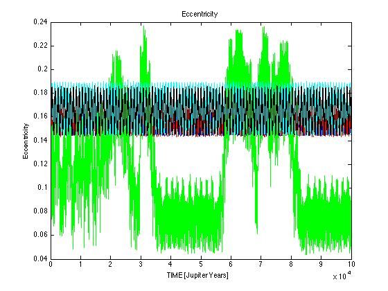
Pythagoras (570-495 BC)

  • Mathematician, philosopher, started a religion
  • all heavenly bodies at whole number ratios
  • ”Harmony of the spheres”

                      Figure: Pythagorean Model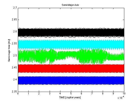
Tycho Brahe (1546-1601)

    • Danish
      astronomer,
      alchemist
    • accurate
      astronomical
      observations, no
      telescope
    • importance of
      data collection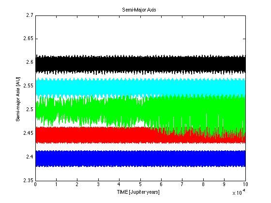
Johannes Kepler (1571-1631)

  • Brahe’s assistant
  • Used detailed data provided by Brahe
  • Observations led to Laws of Planetary Motion
Johannes Kepler (1571-1631)

  • Brahe’s assistant
  • Used detailed data provided by Brahe
  • Observations led to Laws of Planetary Motion
      • orbits are ellipses
      • equal area in equal time
      • T 2 ∝ a3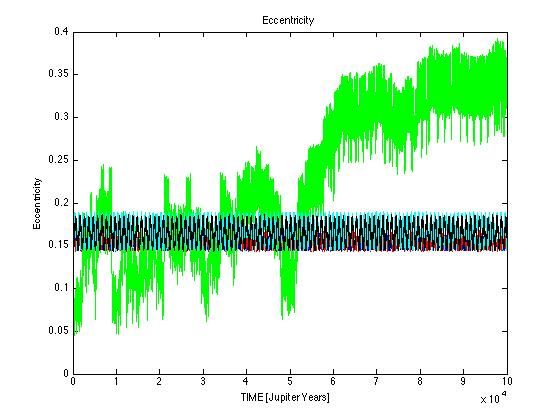
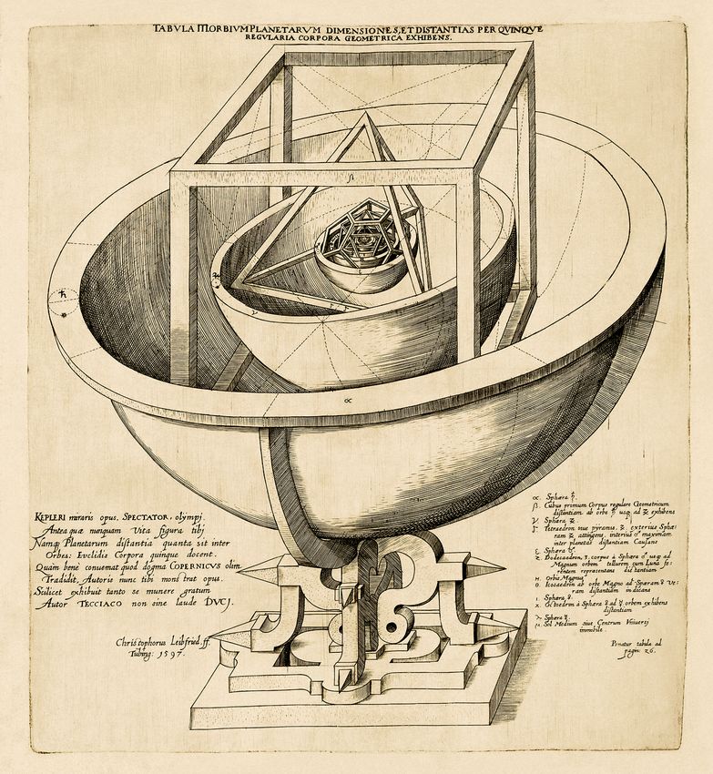
Kepler’s Model

  • Astrologer, Harmonices Mundi
  • Used empirical data to formulate laws

                     Figure: Kepler’s Model
Isaac Newton (1642-1727)
• religious, yet desired a physical mechanism to explain Kepler’s
laws
• contributions to mathematics and science
• Principia
• almost entirety of an undergraduate physics degree
• Law of Universal Gravitation
~ 12 = −G m1 m2 r̂12 .
F
|r12 |2Resonance
• Transition from ratios/ integer spacing to more physical
description, resonance plays a key role in celestial mechanicsResonance
• Transition from ratios/ integer spacing to more physical
description, resonance plays a key role in celestial mechanics
• Commensurability
The property of two orbiting objects, such as planets, satellites, or
asteroids, whose orbital periods are in a rational proportion.Resonance
• Commensurability
The property of two orbiting objects, such as planets, satellites, or
asteroids, whose orbital periods are in a rational proportion.
• Resonance
Orbital resonances occur when the mean motions of two or more
bodies are related by close to an integer ratio of their orbital
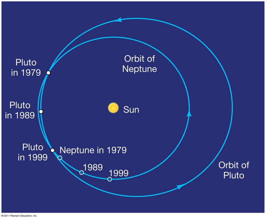
periodsExamples • Pluto-Neptune 2:3 • Ganymede-Europa-Io 1:2:4
Examples
 Cassini division in Saturn’s rings
 1:2 Resonance with Mimas
Kirkwood Gaps
 Daniel Kirkwood (1886)
Kirkwood Gaps

  • Commensurability in the orbital periods cause an ejection by
    Jupiter
  • explanation provided by Kirkwood, using 100 asteroids
  • now thought to exhibit chaotic change in eccentricity
My Goal • To create a simulation of the interactions of Jupiter, the Sun, and ’test’ asteroids • Integrate Newton’s equations of motion in MATLAB over a large time span (≈ 1MY )
Requirements

  1   an idea for what causes orbital resonance
  2   an appropriate integrating scheme
  3   initial conditions for all bodies being considered
Requirements

  1   an idea for what causes orbital resonance
  2   an appropriate integrating scheme
  3   initial conditions for all bodies being considered

  • Start with the Kepler problem
Kepler Problem

  • The problem of two bodies interacting only by a central force
    is known as the Kepler Problem
  • Also known as the 2-body problem
Kepler Problem
m1 m2 m1 m2 (r1 − r2 )
m1 r¨1 = G 2
=G 3
r12 r12
m1 m2 m1 m2 (r2 − r1 )
m2 r¨2 = G 2 = G 3
r12 r12
Center of Mass is stationary/ moves at constant velocityClassic treatment
r¨2 − r¨1 = r̈
r
r̈ + µ 3 = 0
r
G (m1 + m2 ) = µClassic treatment
Considering motion of m2 with respect to m1 gives:
r × r̈ = 0,
which, integrating once, gives
r × ṙ = h
This implies that
the motion in the two-body problem lies in a plane.
Treat this relative motion in polar coordinates (r,θ).Polar form
Using,
r = rr̂
ṙ = rr̂ + r θ̇θ̂
1d 2
r̈ = (r̈ − r θ̇)r̂ + (r θ̇) θ̂,
r dt
one finds the solution:
p
r (θ) = ,
1 + e cos(θ)
h2
where p = µ.Elliptical Orbit
c
Figure: Axes of an ellipse, Eccentricity = aKepler’s Laws
1 The motion of m2 is an ellipse with m1 at one focus
dA h
2 dt = 2 = constant
Figure: Kepler’s 2nd LawKepler’s third law
• From Kepler’s second law, we have dA h
dt = 2 .
• area of ellipse = A = πab
A
• τ = dA
dt
4π 2 a3
3 τ2 = µ , or τ 2 ∝ a3 .N-Body Problem • no analytical solutions for N>2 • computational methods → Euler’s method, Runge-Kutta
N-Body Problem • no analytical solutions for N>2 • computational methods → Euler’s method, Runge-Kutta • need a better method
System

 • N bodies - Sun, Jupiter, asteroids
 • centralized force
 • kinetic and potential energies independent
 • Hamiltonian system
Hamiltonian Formulation

 H(q, p) = T (p) + U(q)

                                 ∂H
                          q̇ =
                                 ∂p
                                 −∂H
                          ṗ =
                                  ∂q
N-Body Hamiltonian
• Hamiltonian is separable, i.e. H = H(q, p, t) = T (p) + U(q)
n
1 X pi2
T =
2 mi
i=1
N X
i−1
X Gmi mj
U=−
|q1 − qj |
i=2 j=1N-Body Hamiltonian
• from Hamilton equations:
pi
q̇i = ∇pi H =
mi
n
X mj (qi − qj )
ṗi = ∇qi H = −Gmi
j6=i
|qi − qj |3Numerical Scheme • best approach → symplectic integrator • designed for solutions to Hamiltonian systems • preserves volume in phase space
Derivation

 To derive the simplectic integrator to be used, compose Euler
 method map
                         qi+1 = qi + dt∇pi H
                       pi+1 = pi − dt∇qi+1 H
 with its adjoint
                        pi+1 = pi − dt∇qi H
                       qi+1 = qi + dt∇pi+1 H
                                         1             dt
 by introducing a ”half time step” i +   2   of size   2.
Derivation
New integrating scheme is now
dt
qi+ 1 = qi + ∇pi H
2 2
pi+1 = pi − dt∇qi+ 1 H
2
dt
qi+1 = qi+ 1 + ∇pi+1 H.
2 2Leapfrog Algorithm
• additional half time-step transforms Euler’s method to
symplectic integrator
• more stable over long integrations
• angular momentum is preserved explicitlyLeapfrog Algorithm
• additional half time-step transforms Euler’s method to
symplectic integrator
• more stable over long integrations
• angular momentum is preserved explicitly
• a simple test of the Leapfrog integrator →Leapfrog Test
Figure: Theoretical SolutionLeapfrog Test
Figure: Numerical SolutionSo far...
• semi-major axis/ orbital period relationship necessary for
resonance
• appropriate integrating scheme
Unresolved...
• Initial conditions for Sun, Jupiter, asteroidsInitial Conditions
• Positions
• sun at origin
• Jupiter at aphelion
• asteroids at perihelion
• Velocities (from ṙ · ṙ )
2 2 1
v =µ −
r aModel
• Integrate orbits of the Sun, Jupiter, and five asteroids
• range of initial semi-major axes, e = 0.15
• initial postions
• Sun at origin
• Jupiter at aphelion
• asteroids at perihelion
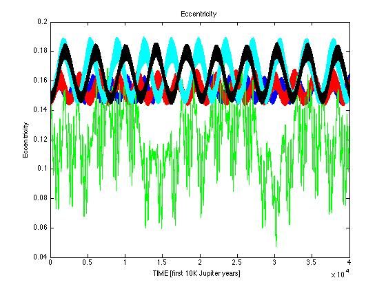
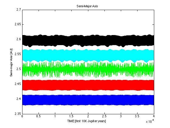
• calculate eccentricities and semi-major axisResults Figure: 3:1 Resonance - 10K Jupiter Years - ∆t = 10.83 days
Results

   Figure: 3:1 Resonance - 10K Jupiter Years - ∆t = 10.83 days
Results

   Figure: 3:1 Resonance - 100K Jupiter Years - ∆t = 10.83 days
Results

   Figure: 3:1 Resonance - 100K Jupiter Years - ∆t = 10.83 days
Results

 Figure: 3:1 Resonance - 100K → 200K Jupiter Years - ∆t = 10.83 days
Results

 Figure: 3:1 Resonance - 100K → 200K Jupiter Years - ∆t = 10.83 days
Further Abstraction
Conclusion

  • resonances play a key role
  • unite pre-scientific revolution → modern science
  • increased computational power → insights into development
    of solar system
References
1 Meteorites may follow a chaotic route to Earth, Wisdom,
Nature 315, 731-733 (27 June 1985)
2 The origin of the Kirkwood gaps - A mapping for asteroidal
motion near the 3/1 commensurability, Wisdom, Astronomical
Journal, vol 87, Mar. 1982
3 Numerical Investigation of Chaotic Motion in the Asteroid
Belt, Danya Rose, University of Sydney Honours Thesis,
November 2008
4 Motion of Asteroids at the Kirkwood Gaps, Makoto
Yoshikawa, Icarus, Vol. 87, 1990
5 The role of chaotic resonances in the Solar System, N. Murray
and M. Holman, Nature, vol. 410, 12 April 2001
6 Introduction to Celestial Mechanics, Jean Kovalevsky, D.
Reidel, 1967
7 Classical Mechanics, John R. TaylorYou can also read