Romanian IO Tables: Updated Series 1989-2018 in Twenty-Sectoral Structure
←
→
Page content transcription
If your browser does not render page correctly, please read the page content below
Romanian IO Tables:
Updated Series 1989-2018 in
Twenty-Sectoral Structure
Emilian Dobrescu

Viorel Gaftea

                                    ABSTRACT

          The INS extended input-output tables were organized into twenty-sectoral
structure, which allows a deeper investigation of the Romanian economy in its evolu-
tion from the centrally planned system to market mechanisms. Integral statistical series
1989-2018 are compacted into three annexes: i) the sectoral shares of output and of
gross value added (Appendix 1); ii) the technical coefficients at current prices (Appen-
dix 2); and iii) the Leontief coefficients at current prices (Appendix 3). Methodological
problems discussed in the previous fourteen-sectoral structure (Romanian Statistical
Review 3/2019) remain valid and are not repeated. As an illustration of the analytical
insights offered by these statistical series, the present paper examines from a dynami-
cal perspective the temporal intensity of sectoral changes, their interdependences, the
main relocations of the output multipliers, structural impulses for changing the ratio of
gross value added to output.
          Key-words: sectoral structure, I-O coefficients, stationarity tests, Granger
causality, output multiplers
          JEL Classification: C12, C67

ROMANIAN IO TABLES: UPDATED SERIES 1989-2018
    IN TWENTY-SECTORAL STRUCTURE
         The previous similar analyses (Dobrescu and Gaftea 2017, 2019)
were built on a fourteen sectoral structure: three sectors from the primary
mega-field of economic activities, five from the secondary, four from tertiary
and two from the quaternary ones.
        1. The present study extends the number of sectors to 20, diminishing
the informational losses induced by the aggregative operations. The sectors
belonging to primary and secondary mega-fields of economic activities,
respectively the sectors 1-8 are identical in both classifications. The other
6 sectors of the previous structure are reorganized into 12 in the new one,

Romanian Statistical Review nr. 3/ 2021                                                3
obtaining a more representative specification of the tertiary and quaternary
mega-fields, which are characterized by a special dynamism under the modern
civilization. The following table describes account correspondence between
twenty-sector and fourteen-sector structures.
Comparative structures used in aggregation of the Romanian IO tables
Table 1
Twenty-sector structure Fourteen-sector structure
● Agriculture, forestry, hunting and fishing (1); ● Agriculture, forestry, hunting and fishing (1);
● Mining and quarrying (2); ● Mining and quarrying (2);
● Production and distribution of electric and ● Production and distribution of electric and
thermal power (3); thermal power (3);
● Food, beverages and tobacco (4) ● Food, beverages and tobacco (4)
● Textiles, leather, pulp and paper, furniture (5); ● Textiles, leather, pulp and paper, furniture (5);
● Machinery and equipment, transport ● Machinery and equipment, transport means,
means, other metal products (6); other metal products (6);
● Other manufacturing industries (7); ● Other manufacturing industries (7);
● Constructions (8); ● Constructions (8);
************************************** **************************************
● Wholesale and retail trade; repair of motor
vehicles, and personal and household goods (9) ● Transports, post and telecommunications (9);
● Transport and storage (10) ● Trading services (10);
● Hotels and restaurants (11) ● Financial services, real estate transactions (11);
● Communications (12) ● Social services (12);
● Information (13) ● Creative services (13); and
●Financial intermediary and insurance (14) ● Professional services (mainly businesses) (14)
● Real estate transactions (15).
● Professional and scientific-technic
activities, administrative and support
services (16)
● Public administration and defense, public
system of the social security (17)
● Education (18)
● Health and social assistance (19)
● Cultural and recreational activities,
spectacles and other services (20)
4 Romanian Statistical Review nr. 3 / 2021The twenty-sector structure of economy can be easily converted into
four mega-fields classification: the primary mega-field includes sectors (1+2+3);
the secondary (4+5+6+7+8); the tertiary (9+10+11+12+14+15+17+19); and
the quaternary (13+16+18+20).
The three annexes detail the statistical series (current prices) for the
entire period 1989-2019 in this new sectoral structure: the sectoral shares in
output and gross domestic value added (Appendix 1), the technical coefficients
(Appendix 2), and the Leontief matrix (Appendix 3). In this way, a large
palette of empirical studies can be developed.
The present study presents only several characteristics of the structural
changes of Romanian economy during its historical transition from centrally
planned system to market mechanisms. Particularly, the following questions
will be especially commented:
▪ temporal intensity of the sectoral changes;
▪ their dynamical interdependences;
▪ the main relocations of the output multipliers;
▪ the structural impulses for changing the ratio of gross value added to
output.
2. Through new sectoral classification, the intensity of structural
changes can be more realistically approximated. For such a purpose, we shall
use (as in the paper from 2019) two measures:
i) moving sectoral structural coefficient
Mssct=((1/m)*∑(shit-shi(t-1))2)0.5 (1) and
ii) referential sectoral structural coefficient
Rssct=((1/m)*∑(shit-rshi)2)0.5 (1a),
where m – is the number of sectors, shit - sectoral shares at time t,
and rshi - sectoral shares adopted as a benchmark (1989 as the last year of the
socialist regime).
2.1. Recomputed for twenty-sectoral structure and for years 1990-
2018, the coefficients (1) and (1a) concerning the productive
sphere of economy - sectoral shares in the output (suffix o) and in
the gross value added (suffix v) - maintain broadly the dynamical
picture identified by fourteen- sectoral structure.
Romanian Statistical Review nr. 3/ 2021 5Moving and referential sectoral structural coefficients for output (suffix o)
and gross value added (suffix v), during the 1990-2018 period
Figure 1
The accentuated structural turbulence during the first part of interval
(signaled already in the previous paper) appears also clearly enough in the
new IO tables. This came from a major peculiarity of the Romanian transition,
when large previous industrial, agricultural and other types of productive
infrastructure sectors were abandoned. The subsequent calmer, from this
point of view, evolution coincided with the implementation of the preliminary
institutional and socio-economic reforms required by the integration of
Romania into European Union. Global financial crisis 2008-2010 and its
consequences re-intensified the structural shifts, mainly regarding the sectoral
ratios of value added to output. The relatively low levels registered during last
years by Mssc are probable temporary, taking into account the expectable new
structural mutations induced by Covid19 pandemic and by the implementation
of EU climatological programs.
6 Romanian Statistical Review nr. 3 / 20212.2. As expected, the supply-side structural changes of Romanian
economy were accompanied by notable modifications concerning
also the utilization of goods and services.
2.2.1. The final consumption characterized by the following temporal
intensity of structural changes (Figure 2).
Moving and referential sectoral structural coefficients for final
consumption (suffix C), during the period 1990-2018
Figure 2
Apart from some shocks registered at the beginning of transition and
along the previous global financial crisis, the moving coefficients oscillate
within a restrained enough band. Compared to the starting point, the structural
changes were however considerable (RsscC).
Romanian Statistical Review nr. 3/ 2021 72.2.3. The gross capital formation shows a different picture from this
point of view. (Figure 3).
Moving and referential sectoral structural coefficients for gross capital
formation (suffix K), during period 1990-2018
Figure 3
The spectacular breaks induced by the initial transformational
processes of the transition to market economy were followed, therefore, by a
stable enough sectoral structure of the investment programs.
8 Romanian Statistical Review nr. 3 / 20212.3. The export (X) and import (M) of Romania also knew profound
structural changes (Figure 3).
Moving and referential sectoral structural coefficients for export
(suffix X) and import (M), during period 1990-2018
Figure 4
Two global features were dominant. On one hand, the external
openness of Romanian economy amplified substantially: as ratio to output,
the foreign trade (sum of export and import) increased from 15-17% during
the first years of transition, to 25% in 2000 and to 46% in 2018. On the other
hand, this trend was associated with important deficits of the foreign trade
balance.
3. Treated themselves as time series, the coefficients Mssc allow
to identify some dynamic interdependences among the structural change
intensities in different spheres of economic activity. In our case, of great
interest are such possible connections between the production and utilization
of goods and services, respectively between Mssco, and the corresponding
indicators for final consumption, gross capital formation, export and import.
With this aim, it will be used the Granger causality test (Granger 1969), whose
application is conditioned by the stationarity of the examined series.
Romanian Statistical Review nr. 3/ 2021 93.1. Taking into account the diversity of the cognitive specificities
belonging to statistical procedures conceived in this field,
there will be used a set of unit root tests (Dickey and Fuller
1981, Phillips and Perron 1988, Kwiatkowski et al. 1992, Ng
and Perron 1994, Gujarati and Porter 2009, Patterson 2011,
Patterson 2012). We used: Augmented Dickey-Fuller (ADF),
Phillips-Perron (PP), DF-GLS (developed by Elliott-Rothenberg-
Stock), Kwiatkowski-Phillips-Schmidt-Shin (KPSS), Elliott-
Rothenberg-Stock point optimal (ERS), Ng-Perron (NgP) in
four variants (MZa, MZt, MSB, MPT), and Breakpoint. Table 2
synthetizes the null hypothesis probabilities obtained for all five
mentioned time-series.
Stationarity tests for the moving sectoral structural coefficients of output
and utilization of goods and services - Probability of the null hypothesis
Table 2
Statistic test Null hypothesis Mssco MsscC MsscK MsscX MsscM
Series has a unit
Augmented Dickey-Fuller 0.0032 0.0004 0.0731 0.0054 0.0446
root
Series has a unit
Phillips-Perron 0.003 0.0004 0.0986 0.0059 0.0566
root
Elliott-Rothenberg-Stock Series has a unit under under under under under
DF-GLS root 0.01 0.01 0.01 0.01 0.01
Kwiatkowski-Phillips- Series is 0.01- 0.01- 0.01- 0.01- 0.01-
Schmidt-Shin stationary 0.05 0.05 0.05 0.05 0.05
Series has a unit under 0.01-
Elliott-Rothenberg-Stock over 0.1 over 0.1 0.05-0.1
root 0.01 0.05
Series has a unit
Ng-Perron
root
0.01- under 0.01- 0.01- 0.01-
Variant MZa
0.05 0.01 0.05 0.05 0.05
0.01- under 0.01- 0.01- 0.01-
Variant MZt
0.05 0.01 0.05 0.05 0.05
0.01- under 0.01- 0.01- 0.01-
Variant MSB
0.05 0.01 0.05 0.05 0.05
0.01- under 0.01- 0.01- 0.01-
Variant MPT
0.05 0.01 0.05 0.05 0.05
Series has a unit under under under under
Breakpoint 0.0448
root 0.01 0.01 0.01 0.01
Therefore, the probability of null hypothesis does not reject the
stationarity of the respective series in 8 applications for Mssco, 9 for MsscC,
7 for MsscK, 8 for MsscX, and 7 for MsscM. Such a proportion justifies, in
our opinion, the utilization of Granger causality test in its standard version.
10 Romanian Statistical Review nr. 3 / 20213.2. Applied on the relationship between output and its main destinations
– domestic absorption and foreign trade - the results of Granger
causality test for one and two lags are presented in Table 3.
Granger causality test, sample 1989-2018, for one and two lags
Table 3
Lags 1 Lags: 2
Null Hypothesis: Obs F-Statistic Prob. Obs F-Statistic Prob.
Mssco does not Granger
28 0.24274 0.6265 27 5.68776 0.0102
Cause MsscC
MsscC does not Granger
0.00534 0.9424 1.00846 0.381
Cause Mssco
Mssco does not Granger
28 3.42541 0.0761 27 3.04465 0.068
Cause MSCCK
MSCCK does not Granger
5.5223 0.027 1.38847 0.2705
Cause Mssco
Mssco does not Granger
28 0.13288 0.7185 27 0.0398 0.9611
Cause MsscX
MsscX does not Granger
0.6277 0.4357 0.26696 0.7682
Cause Mssco
Mssco does not Granger
28 4.23263 0.0502 27 6.16053 0.0075
Cause MsscM
MsscM does not Granger
14.9554 0.0007 4.17151 0.0291
Cause Mssco
These results do not confirm the tempter impression that structural
changes intensity of output could come from the final consumption or export
impulses. Stronger appears to be the connection of output with gross capital
formation. What has to be especially outlined is the bilateral interdependence
between output and import.
4. Among powerful analytical tools offered by the IO tables, the output
multipliers (scLi) have a special role. Approximating the global output generated
by the entire economy for ensuring an increase by unity of the final resources of
given sector i, these are equal to sum-columns of the Leontief matrix (Lij):
scLi=∑jLij (j=1, 2,…, n) (2)
Economically, therefore, the output multipliers reflect not only the
direct, but also the propagated inter-branches productive flows (Dobrescu
1970, Leontief 1974, Leontief 1986, Okuyama et al. 2004, Pilat and Wölfl
2005, Eurostat, European Commission 2008, Hall 2009, Miller and Blair 2009,
D’Hernoncourt et al. 2011, Bess and Ambargis 2011, Lazarov and Kocovski
2016, Hughes 2018, The Scottish Government 2020).
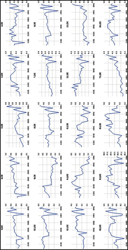
4.1. Figure 5 displays an overview about dynamics of output-
multipliers scLi in Romanian economy.
Romanian Statistical Review nr. 3/ 2021 11Output-multipliers (scLi) during the period 1989-2018
Figure 5
12 Romanian Statistical Review nr. 3 / 2021The rather turbulent evolution of output-multipliers should come as no
surprise since they cumulate an extremely large spectrum of transformations
– institutional and technologic-managerial, not avoiding the operational
behaviors of economic agents and even accounting systems. Despite this
“whirling” picture, some tendential features have to be noted.
4.2. Evolution of the output multipliers takes place between some
limits, as revealed by Figure 6.
Limits of variation of scli produced during 1989-2018
Figure 6
Statistical analysis discloses some notable aspects. As time series,
scLmax is clearly stationary: it is confirmed by 9 tests (ADF, PP, ERSDF-
GLS, KPSS, NgP all four variants, Breakpoint); only ERS is negative). The
case of scLmin is somehow different: ERS, NgP, and breakpoint tests do not
accredit the stationarity; it is however accepted by ERSDF-GLS and KPSS,
and at limit by ADF (0.0673 - null hypothesis probability) an PP (0.0717). The
autocorrelation analysis signals a certain interdependence among data scLmax
and scLmin series (Table 4).
Romanian Statistical Review nr. 3/ 2021 13Autocorrelation of scLmax and scLmin series
Table 4
scLmax scLmin
Lags AC PAC Q-Stat Prob AC PAC Q-Stat Prob
1 0.253 0.253 2.1142 0.146 0.607 0.607 12.201 0
2 0.121 0.061 2.6132 0.271 0.381 0.019 17.174 0
3 0.268 0.24 5.1586 0.161 0.215 -0.037 18.818 0
4 -0.122 -0.276 5.71 0.222 0.097 -0.038 19.169 0.001
5 -0.092 -0.03 6.0357 0.303 0.083 0.07 19.431 0.002
6 0.089 0.093 6.351 0.385 0.038 -0.039 19.488 0.003
7 0.113 0.224 6.8847 0.441 -0.03 -0.079 19.525 0.007
8 -0.031 -0.154 6.9271 0.545 -0.115 -0.106 20.106 0.01
BDS test (Broock et al. 1996) enforces the conclusion that both series
scLmax and scLmjn are not independent identically distributed (iid) series.
BDS test applied on scLmax and scLmin series
Table 5
Dimension scLmax scLmin
Norm. Bootstrap BDS Norm Bootstrap
BDS Statistic
Prob. Prob. Statistic Prob. Prob.
Fraction of pairs
2 0.065307 0.0001 0.0148 0.081954 0 0.0012
3 0.128987 0 0.0052 0.132149 0 0.0016
4 0.168815 0 0.0024 0.156251 0 0.0022
5 0.228047 0 0.0006 0.15622 0 0.0054
6 0.251139 0 0.0002 0.145564 0 0.009
Standard deviations
2 0.129814 0 0 0.088276 0 0
3 0.186813 0 0 0.091553 0 0.001
4 0.213276 0 0 0.077932 0 0.002
5 0.218998 0 0 0.050943 0 0.0044
6 0.215737 0 0 0.03226 0 0.0092
Fraction of range
2 0.129814 0 0 0.013589 0 0.1266
3 0.186813 0 0 0.030327 0 0.1004
4 0.213276 0 0 0.050535 0 0.0872
5 0.218998 0 0 0.074534 0 0.0748
6 0.215737 0 0 0.102629 0 0.0624
14 Romanian Statistical Review nr. 3 / 2021There exist, therefore, enough reason for treating both scLmax and
scLmin series as auto-regressive processes. With this end, for the series
scLmax and scLmin there was selected a VAR system with as high as possible
number of lags in order to take into account peculiarities of the sample data
under stability VAR restriction. The following equations were retained:
scLmax = 0.739275*scLmax(-1) + 0.352509*scLmax(-2) -
0.176618*scLmax(-3) + 0.063871*scLmax(-4) - 0.095537*scLmax(-5)
- 0.060627*scLmax(-6) - 0.02749*scLmax(-7) - 0.120791*scLmax(-8) +
0.200991*scLmin(-1) - 0.053133*scLmin(-2) - 0.042201*scLmin(-3) +
0.134704*scLmin(-4) - 0.329895*scLmin(-5) + 0.307413*scLmin(-6) +
0.184198*scLmin(-7) - 0.242667*scLmin(-8) + 0.755140 (3a)
scLmin = 0.245675*scLmax(-1) - 0.167622*scLmax(-2) -
0.103779*scLmax(-3) + 0.148758*scLmax(-4) + 0.004381*scLmax(-5) +
0.093199*scLmax(-6) - 0.011095*scLmax(-7) - 0.055810*scLmax(-8) +
0.2316025*scLmin(-1) + 0.012499*scLmin(-2) + 0.075238*scLmin(-3)
- 0.281911*scLmin(-4) - 0.101835*scLmin(-5) + 0.157412*scLmin(-6) -
0.033316*scLmin(-7) - 0.12872*scLmin(-8) + 1.075381 (3b)
Observing the VAR stability condition, these equations were simulated
by successive post-sample iterations. The resulted difference
dscL=scLmax-scLmin (4)
approximates the band within which the output multipliers are moving. Figure
7 plots the stabilizing tendency of this band in hypothetical absence of new
shocks.
Romanian Statistical Review nr. 3/ 2021 15Estimated band (dscL=scLmax-scLmin) of the output multipliers
evolution
Figure 7
4.3. As expected, such a dynamic process as transition involves a
changing sectors hierarchy, depending on their output-multipliers
size. Table 6 presents the number of observations in which the
sector i (labeled on columns) places on rank j (on rows).
16 Romanian Statistical Review nr. 3 / 2021Number of observations in which the sector i places on rank j
Table 6
Rank /
j Sum
Sector
I 1 2 3 4 5 6 7 8 9 10 11 12 13 14 15 16 17 18 19 20
1 4 10 2 7 7 30
2 1 7 6 5 4 7 30
3 2 1 3 4 3 5 5 6 1 30
4 3 7 3 8 2 1 5 1 30
5 1 6 9 9 1 3 1 30
6 1 5 1 2 2 5 3 2 5 4 30
7 2 1 1 4 2 3 1 10 3 1 2 30
8 6 1 1 4 2 1 1 1 8 2 1 2 30
9 6 2 5 3 1 7 3 3 30
10 6 3 1 3 1 3 1 3 9 30
11 1 1 1 3 1 7 3 3 2 2 6 30
12 4 1 1 2 1 4 2 7 2 1 1 2 1 1 30
13 3 2 1 5 2 6 4 1 4 1 1 30
14 6 2 3 8 1 3 1 2 2 1 1 30
15 1 4 9 5 1 1 2 1 1 5 30
16 1 4 5 7 1 3 4 1 1 3 30
17 2 4 8 2 3 2 3 1 1 2 2 30
18 7 3 2 8 2 5 2 1 30
19 1 11 1 13 2 1 1 30
20 10 1 6 13 30
Sum 30 30 30 30 30 30 30 30 30 30 30 30 30 30 30 30 30 30 30 30
The greatest output multiplier (rank 1) belonged, therefore, ten years
to sector 14, 7 to sector 17, and again 7 to sector 18. At opposite side, the
lowest output multiplier (rank 20) was registered 13 times for sector 7, 10
for sector 3, and 6 for sector 6. Hierarchy of these sectoral output multipliers
can be especially useful in the analysis and projection of the macroeconomic
consequences of different structural changes.
5. An important problem concerns the impact of the sectoral
distribution of output on the ratio of gross value added to output, named
rgva. This approximates globally the adding value rate (to used productive
inputs) of different economic activities, independent on sources inducing
it: technological innovations, managerial improvements, relative prices
modifications.
Romanian Statistical Review nr. 3/ 2021 175.1. Figure 8 plots dynamics of rgva at level of entire Romanian
economy,
Evolution of rgva during 1989-2018
Figure 8
The initial growth of rgva has resulted probably from the initial
abrupt liberalization of economic activity, associated with the deep shifts in
the relative intersectoral prices and a drastic compression of the mining and
other primary branches. This first phasis is followed by another - long enough
of slightly increasing and mainly stabilizing trend, interrupted by the global
financial recession. The post-crisis recovery must be cautiously taken into
consideration because the data do not comprise Covid19 pandemic years.
5.2. Sectoral rgvai have characterized by several evolutive patterns.
Five of them (4, 5, 7, 15, 17) knew an ascending trend, while others - again
five (1, 9, 12, 13, 14) registered a contrary trend; all the rest traversed more or
less accentuated oscillations. As an average on the whole interval, the sectoral
rgva are distributed as follows: the median group (rgva between 0.4-0.6)
comprises 11 sectors (1, 2, 5, 8, 9, 10, 11, 12, 16, 19, 20), the lowest group
(rgva under 0.4) comprises four sectors (3, 4, 6, 7), and the other five (13, 14,
15, 17, 18) belong to the superior one (rgva over 0,6).
18 Romanian Statistical Review nr. 3 / 20215.3. Dynamically, the ratio of gross value added to output (rgvat) can
be interpreted as a function of impulses coming from the changes
of the sectoral rates as such (rgvai) and from modification of the
sectoral distribution of output (rgvaqi). The first type of influences
is aggregated into rgvar, and the second one into rgvac. In what
proportions the rgva evolution was determined by these two
types of influences – it would be certainly a question of interest.
Therefore:
rgvat=f(rgvart, rgvaqt, resrqt, ut) (5)
rgvart=Σ(rgvait*shqi(t-1)) i=1, 2,…,n) (6)
rgvaqt=Σ(rgvai(t-1)*shqit) i=1, 2,…,n) (7)
where i symbolizes the code of sector.
In accordance with the stated analytical purpose – that is the best
possible approximation of proportion in which rgvar and rgvaq are influencing
rgva – a strictly bifactorial linear specification of (5) would be preferable. The
series rgva, rgvar, and rgvaq are not stationary in levels.
Regarding rgva, only PP and KPSS are accepting the stationarity
in level, all the rest of the processed tests suggesting opposite conclusion.
The situation is not significantly different nor for rgvar (with ADF, PP, and
KPSS favorable) or for rgvaq (with PP and KPSS). The first order differences
(prefix d) are, instead, undoubtedly stationary: ERS procedure is the only one
ambiguous for drgva. Consequently, the relationship (5) was estimated in
differences, with the following results:
Dependence ofd rgva on drgvar and drgvaq
Table 7
Variable Coefficient Std. Error t-Statistic Prob.
C -0.00052 0.001618 -0.32233 0.7499
drgvar 0.798022 0.090976 8.771832 0
drgvaq 0.191501 0.080164 2.388877 0.0248
R-squared 0.773947 Mean dependent var 0.003575
Adjusted R-squared 0.755863 S.D. dependent var 0.016521
S.E. of regression 0.008163 Akaike info criterion -6.67745
Sum squared resid 0.001666 Schwarz criterion -6.53471
Log likelihood 96.48425 Hannan-Quinn criter. -6.63381
F-statistic 42.79676 Durbin-Watson stat 3.063668
Prob(F-statistic) 0
Therefore, at the level of the entire economy, the variation of rgva is
decisively conditioned by changes of its sectoral levels, and only subsidiarily
by the modification of its sectoral distribution of output as such.
Romanian Statistical Review nr. 3/ 2021 196. Authors are grateful to Prof. Tudorel Andrei and Dr. Adriana
Ciuchea for their competent implication in building the Romanian IO tables
and in sustaining our efforts to realize the research project presented in
Romanian Statistical Review 3/2019.
References
1. Bess, R. and Ambargis Z.O. (2011), “Input-Output Models for Impact Analysis:
Suggestions for Practitioners Using RIMS II Multipliers”, Presented at the 50-
th Southern Regional Science Association Conference March 23-27, 2011 New
Orleans; https://www.bea.gov/system/files/papers/WP2012-3.pdf (Acc. 12 July
2021))
2. Broock, W. A., Scheinkman, J.A., Dechert, W.D. and LeBaron B. (1996), “A test for
independence based on the correlation dimension”, Econometric Reviews, 15:3, pp.
197-235, DOI: 10.1080/07474939608800353; http://it-girls.informatik.uni-frankfurt.
de/software/MI2/papers/bds96.pdf (Acc. 15 July 2021).
3. D’Hernoncourt, J., Cordier, M., and Hadley, D. (2011), Input-Output Multipliers
– Specification sheet and supporting material, Spicosa Project Report, Université
Libre de Bruxelles – CEESE, Brussels; http://www.coastal-saf.eu/output-step/pdf/
Specification%20sheet%20I_O_final.pdf (Acc. 12 July 2021).
4. Dickey D.A., Fuller W.A. (1981): “Likelihood ratio statistics for autoregressive
time series with a unit root”, Econometrica Econometrica 49(4),1057-72,
DOI: 10.2307/1912517.
5. Dobrescu, E. (1970), “Inter-Branches Balance – An Instrument of Structural
Analysis of Economy”, Economic Computation and Economic Cybernetics Studies
and Research, 4, 27-51.
6. Dobrescu, E. and Gaftea V. (2017), “The sectoral structure of an emergent economy
in light of I-O analysis”, 25th International Input-Output Association Conference,
June 19-23, 2017, Atlantic City, New Jersey, USA; https://www.researchgate.net/
publication/329092827_The_sectoral_structure_of_an_emergent_economy_in_
light_of_I-O_analysis_-_Romania (Acc. 28 July 2021).
7. Dobrescu, E. and Gaftea V., (2019), “Input-Output Coeffi cients of the Romanian
Economy - Annual Data 1989-2016, Current Prices -“, Romanian Statistical Review
3, 73-89; https://www.revistadestatistica.ro/wp-content/uploads/2019/09/A7_RRS-
3_2019.pdf, (Acc. 28 July 2021).
8. Eurostat, European Commission (2008), “Eurostat Manual of Supply, Use and Input-
Output Tables”; https://ec.europa.eu/eurostat/documents/3859598/5902113/%20
KS-RA-07-013-EN.PDF/b0b3d71e-3930-4442-94be-70b36cea9b39?version=1.0.
9. Granger, C.W.J. (1969), “Investigating Causal Relations by Econometric
Models and Cross-spectral Methods”, Econometrica. 37 (3), 424–
438, doi:10.2307/1912791. JSTOR 1912791.
10. Gujarati, D.N. and Porter, D.C. (2009), “Basic Econometrics”, Fifth Edition,
McGraw-Hill/Irwin; https://cbpbu.ac.in/userfiles/file/2020/STUDY_MAT/ECO/1.pdf
11. Hall, R.E. (2009), “By how much does GDP rise if the government buys more
output?”, NBER Working Paper, 15496. Cambridge, MA: National Bureau of
Economic Research; https://www.nber.org/system/files/working_papers/w15496/
w15496.pdf (Acc. 10 July 2021).
12. Hughes, D.W. (2018), “A Primer in Economic Multipliers and Impact Analysis Using
Input-Output Models”; https://extension.tennessee.edu/publications/Documents/
W644.pdf (Acc. 11 July 2021).
20 Romanian Statistical Review nr. 3 / 202113. Kwiatkowski, D., Phillips, P.C.B., Schmidt, P. and Shin, Y. (1992), “Testing the
null hypothesis of stationarity against the alternative of a unit root: How sure are we
that economic time series have a unit root?”, Journal of Econometrics, 54(1–3), 159-
178; https://www.sciencedirect.com/science/article/abs/pii/030440769290104Y
(Acc. 27 July 2021).
14. Lazarov, D., Kocovski, M. (2016), “Empirical estimation of the multiplicative
effects of steel industry in Macedonia by using input-output model”, UTMS
Journal of Economics, ISSN 1857-6982, 7(1), 25-35; https://www.econstor.eu/
bitstream/10419/174141/1/869228161.pdf (Acc. 10 July 2021).
15. Leontief, W. W. (1974), “Essais d’économiques”. Ed. Calman Lévy, pp.133-157.
Available in English in: Input-output Analysis, Input-output Economics, New York
Oxford University Press, 1966; - Environmental repercussions and the Economic
Structure : An Input-Output Approach, published in The Review of Economics and
Statistics, Vol. LII, n°3, August 1970, Copyright by the President and Fellows of
Harvard College; published as well in Robert and Nancy DORFMAN, Economics of
the Environment, W.W. Norton & Co Inc, 1972.
16. Leontief, W. W. (1986), “Input–output economics”, 2nd edition, New York, Oxford
University Press.
17. Miller, R. E. and Blair, P. D. (2009), “Input-Output Analysis: Foundations and
Extensions”, 2 edition [e-book], Cambridge University Press.
18. Ng, S. and Perron P. (1994), “Unit Root Tests ARMA Models with Data Dependent
Methods for the Selection of the Truncation Lag”, Cahiers de recherche from Centre
interuniversitaire de recherche en économie quantitative, CIREQ.
19. Okuyama, Y., Sonis, M. and Hewings, G.J.D. (2004), “Typology of structural
change in a regional economy: a temporal inverse analysis”, REAL 04-T-12; http://
citeseerx.ist.psu.edu/viewdoc/download?doi=10.1.1.493.5913&rep=rep1&type=p
df (Acc. 12 July 2021).
20. Patterson K. (2011), “Unit Root Tests in Time Series”, Volume 1: Key Concepts and
Problems. Palgrave Texts in Econometrics. Palgrave Macmillan.
21. Patterson K. (2012), “Unit Root Tests in Time Series”, Volume 2: Extensions and
Developments. Palgrave Texts in Econometrics. Palgrave Macmillan; 2012. ISBN:
9780230250260.
22. Phillips P.C.B. and Perron P. (1988), “Testing for a unit r in time series regression”,
Biometrika 75, 335–346.
23. Pilat, D., Wölfl A. (2005), “Measuring the Interaction Between Manufacturing
and Services”, OECD Science, Technology and Industry Working Papers
2005/05, https://dx.doi.org/10.1787/882376471514, https://www.oecd-ilibrary.org/
docserver/882376471514.pdf?expires=1627832036&id=id&accname=guest&chec
ksum=5F33848F3829E8839A428953D27272DA, (Acc. 20 September 2016).
24. The Scottish Government (2020), “Scottish Input-Output Tables: Methodology
Guide”, Version 5; https://www.google.com/search?q=%E2%80%9CScottish+Input-
Output+Tables%3A+Methodology+Guide%E2%80%9D%2C+Version+5&oq=%E2
%80%9CScottish+Input-Output+Tables%3A+Methodology+Guide%E2%80%9D%
2C+Version+5&aqs=chrome..69i57.808j0j7&sourceid=chrome&ie=UTF-8 (Acc. 28
July 2021).
Romanian Statistical Review nr. 3/ 2021 21You can also read