Land Erosion and Coastal Home Values - Scott Below, Eli Beracha, and Hilla Skiba

Land Erosion and Coastal Home Values

                     Scott Below, Eli Beracha, and Hilla Skiba

Abstract: This paper studies transaction data on coastal homes in an area where continuous land
erosion has been identified and well-documented. We employ a variety of hedonic regressions to
measure the extent to which coastal land erosion is capitalized into the value of waterfront
residential properties. The empirical findings are consistent with our theoretical model that
illustrates the effect of long run discounting on property values. Our results suggest that the rate
of land erosion negatively affects the value of coastal properties. However, the negative effect of
land erosion on transaction prices is only evident when the ratio of the property’s distance from
the shore to the rate of erosion is sufficiently low. Moreover, we provide evidence that nonlocal
buyers pay a premium for properties compared with local buyers and that levels of income,
education and housing value in the area of the buyers’ permanent home address are all correlated
with the purchase price.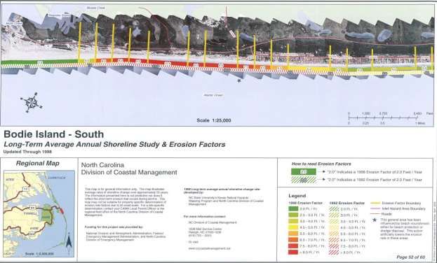

1. Introduction

        Coastal regions in the United States are some of the most densely populated and

developed areas in the nation. According to the National Oceanic and Atmospheric

Administration (NOAA), over the last few decades the proportion of the US population that lives

near the coasts grew faster than the population in the remaining areas. In fact, over 50% of the

US population currently lives in coastal areas, that represent just 17% of the land area in the

contiguous US. Since World War II, the rapid influx of people to the coasts has served as an

engine for growth in the coastal economies and has contributed to above average increases in

home prices along both coasts and the Gulf of Mexico.

        While many people find coastal areas to be attractive places to live, coastal shorelines,

which are commonly viewed as the most desirable locations, are vulnerable to a variety of

environmental hazards. High-energy storms such as hurricanes and nor'easters, combined with

rising sea levels, threaten many shoreline communities. Catastrophic meteorological events, such

as seen with hurricanes Katrina and Sandy, have been associated with monetary losses reaching

tens of billions of dollars and costing hundreds of human lives.1 In light of these recurring

meteorological catastrophes, decisions regarding whether to rebuild in some of the most severely

damaged areas, such as areas along the Gulf Coast and Jersey Shore, have been complex and

contentious.

        This paper examines the extent to which shoreline erosion is being capitalized into the

price of residential coastal real estate. Few papers in the extant literature have studied the price

impact of erosion on real estate, and those that have are typically limited by small and

incomplete datasets. This study contributes to the research on the capitalization of catastrophic

1
  The monetary costs of hurricane Katrina and hurricane Sandy were estimated at $81B in 2005 and $68B in 2013,
respectively. The death tolls reported to be associated with each of these hurricanes were 1,833 and 286
respectively.

                                                       1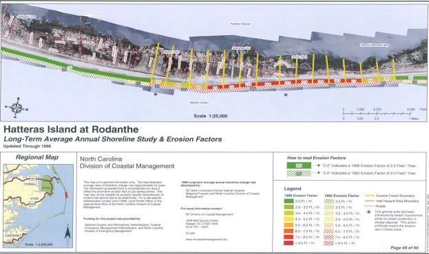

risk into property prices by addressing several of the key shortcomings within the current

literature. First, we address the small sample size problem common in many previous papers by

utilizing a large sample of transactions spanning an extended period of time. Second, we

combine data from a number of sources to create a dataset that includes property level

transaction data, detailed property characteristics, and shoreline erosion data. In addition to

identifying the common property-specific factors that have been shown to impact transaction

prices, we also record the actual distance of each house from the water in feet and match each

property with the estimated shoreline erosion rate at that specific location. Moreover, we utilize

identifying information on the buyers of the properties, including the buyers’ permanent home

addresses, in order to study whether local buyers of the properties in our sample pay a different

price compared with nonlocal buyers. The buyer data also allow us to examine the driving

factors behind any price differential. Fifth, we present a theoretical framework for discounting

near and distant disastrous events. Finally, using the dates of specific named storms, we

investigate whether the capitalization of erosion risk immediately following severe storms varies

from the capitalization of the erosion risk during “normal” times.

       All real estate is at risk from natural disasters, but in contrast to events like tornadoes,

earthquakes, and floods, which are indiscriminate and largely unpredictable, beach erosion is an

endless process whose progress can be observed and measured over time. For example, consider

a house located 150 feet from the mean high tide line of a shoreline that is estimated to be

receding at an average rate of five feet per year. Armed with this information, a potential buyer is

able to develop a rough estimate of how long the property could remain habitable (in the absence

of a catastrophic storm and barring artificial measures undertaken by the state, local, or federal

governments to slow the natural erosion process). Exposure to a progressive, continuous erosion

                                                 2

process differs significantly from exposure to risky meteorological events that occur

sporadically, with a high degree of uncertainty. Most importantly, estimates of long run shoreline

erosion rates are publicly available by location and agents’ fiduciary responsibility mandates

disclosure of such material information prior to the sale. In addition, insurance premiums may

also signal the risks to which a property is exposed. As a result, we should expect rational market

participants to at least partially capitalize erosion risk into their buying decisions and,

consequently, property prices.

        Our findings from transaction level data on coastal homes suggest that land erosion risks

are at least partially capitalized into the prices of waterfront residential properties, and the

empirical findings are consistent with the predictions of our theoretical models. We find that

properties located closer to the ocean within areas exposed to the highest erosion rates are

associated with negative relative price premiums. However, we also find this negative effect to

be statistically significant only if the ratio of the property’s distance from the shoreline to the rate

of erosion (henceforth, the distance-to-erosion ratio) is sufficiently low. In other words, it

appears that erosion risk is not capitalized into property prices until the threat of the property loss

becomes imminent. Additionally, and consistent with the existing literature, we find evidence

that nonlocal homebuyers, on average, pay a price premium for properties compared with local

buyers. Also consistent with the existing literature, we show that the relative price premium

appears to be driven by a price anchoring bias and higher transaction costs. However, we provide

new evidence that buyers’ income and education level are also correlated with the price they pay.

        Given that a large share of the US population lives in coastal areas, we believe the results

of this study are important for a large number of homebuyers and real estate investors, as well as

for the various governmental agencies involved in mitigating the impacts of natural disasters.

                                                   3

The rest of this paper is organized in the following way. Section 2 motivates our research

by discussing the threats associated with land erosion in more detail and reviewing some of the

relevant existing literature. Section 3 presents our theoretical model and develops the hypotheses.

Section 4 describes our dataset and the methodology used in the empirical analysis. Section 5

presents the results of the analysis and Section 6 concludes.

2. Motivation for the Study, Contribution and Literature Review

2.1. Motivation and Contribution

         The barrier islands of the mid-Atlantic coast are unique in that they are made up solely of

sand and clay and are not supported by underlying bedrock. This unique composition, combined

with strong ocean currents and frequent severe storms, means these Outer Banks islands migrate

more than virtually any other coastal area in the United States.2

         While it is possible to artificially protect some shoreline areas via periodic beach

nourishment (i.e. placing new sand onto eroded beaches) or by the installation of seawalls or

groins, the costs can be prohibitive. In addition, hardened structures like seawalls and groins

merely shift the erosion issues down the beach to become someone else’s problem. As a result,

installation of hardened structures along the North Carolina coast is illegal.

         It is estimated that beach nourishment in North Carolina has cost more than $3.8 million

per mile of shoreline since the nourishment programs began, and North Carolina is not unique in

this regard. For example, The Program for the Study of Developed Shorelines (PSDS) estimates

that New Jersey has spent more than $11 million per mile of shoreline in beach nourishment

2
  Riggs, Stanley R., et al, "The Battle for North Carolina's Coast-Evolutionary History, Present Crisis, & Vision for
the Future." The University of North Carolina Press, 2011, pg. 3.

                                                          4

programs (pre-hurricane Sandy) and Florida in excess of $4.6 million per mile of shoreline.3

Geologists argue that rising ocean levels will only increase the demand for beach nourishment

programs going forward and that artificially protecting shorelines in this fashion is an

unwinnable battle, in addition to being prohibitively expensive.

         This study furthers current knowledge of the capitalization of catastrophic risk into

property prices by addressing several of the shortcomings in the extant literature. Specifically,

we address many of the data limitations common in the previous research by analyzing a large

sample of transactions that span an extended period of time. We are also able to consider each

individual property’s precise distance to the water in combination with the average annual

erosion rate of the shoreline in front of each home in the sample. This two-pronged approach

allows us to isolate the effects of proximity to the water from the effect of erosion rates on

property values.

         Due to the topography of the area we explore, we are also able to compare oceanfront

properties to inland and soundfront properties. Like oceanfront properties, soundfront properties

enjoy direct access to the water and waterfront views, but are not subject to the same level of

erosion risk and may even be beneficiaries of accretion. Finally, we are also able to investigate

the extent to which the nonlocal price premium is related to the levels of income and education at

the buyers’ place of origin, in addition to housing price levels that have been considered in the

existing literature.

3
  Source: Program for the Study of Developed Shorelines’ (PSDS) Beach Nourishment Database. All estimates are
in 2012 dollars and based on historical aggregates beginning with the first nourishment event in the dataset, which
took place in the late 1920s.

                                                         5

2.2. Literature Review

        Many existing studies explore the effect of exogenous environmental factors on coastal

real estate valuation. With regard to location, the literature provides consistent evidence that

waterviews materially enhance property values (Kulshreshtha and Gillies 1993; Lansford and

Jones 1995; Benson, Hansen, Schwartz and Smersh 1998; Pompe and Rinehart 1999; Bond,

Seiler and Seiler 2002; Bin, Crawford, Kruse and Landry 2008; Wyman, Hutchinson and Tiwari

2014, among others). On the other hand, studies focusing on coastal flood hazards (Skantz and

Strickland 1987; Harrison, Smersh and Schwartz 2001; Hallstrom and Smith 2005; Bin, Kruse

and Landry 2008; Bin, Crawford, Kruse and Landry 2008, for example) consistently find that

higher susceptibility to temporary flooding or rising sea levels negatively impacts coastal

property values. A recent paper by Turnbull, Zahirovic-Herbert and Mothorpe (2013) also

illustrates that higher flood risk not only affects transaction prices, but also negatively impacts

liquidity.

        Some papers have examined the impact of proximity to the water on the price of

waterfront properties, but the evidence so far is conflicting. Studies by Gopalakrishnan, Smith,

Slott and Murray (2010), Landry, Keeler and Kriesel (2003), and Pompe and Rinehart (1995)

find evidence for the capitalization of beach width into property prices. However, the results

from these studies vary widely, with the marginal willingness to pay for a one-foot increase in

beach width ranging from $70 to $8,000. In contrast, a recent study by Ranson (2012) finds that

beach width has little impact on housing prices in general, except in the case of some highly

eroded beaches. The highly variable and dissimilar results of these studies are likely driven, at

least in part, by the difficulty of gathering reliable data on the main factors affecting a buyer’s

willingness to pay for beach width. While some of these studies have precise information on the

                                                6

distance of the properties from the shoreline, they fail to account for differences in coastal

dynamics across locations and properties. In particular, the distance from the shore should be

considered together with the rate at which the shoreline is eroding. The fact that previous

research has not considered shoreline loss rates may partially explain the disparity in the

conclusions of the studies.

       Pompe and Rinehart (1999) as well as Landry, Keeler and Kriesel (2003) recognize that

the capitalization of land erosion rates into transaction prices depend on market participants’

knowledge of the coastal dynamics and their expectations regarding future artificial coastal

management actions. However, these studies do not distinguish between participants with

varying levels of information.

       Our study also investigates price premiums paid by different buyer types. In previous

papers, Lambson, McQueen and Slade (2004) investigate the price premium paid by nonlocals,

in general, relative to the price paid by local buyers for apartments in the Phoenix area. The

authors conclude that the relative nonlocal price premium is a result of an anchoring bias and

higher search costs. In addition, Hardin and Wolverton (1999) show evidence for a price

premium related to buyer type. Specifically, they show that REITs pay acquisition premiums

over other types of buyers.

       The paper also relates to the literature on capitalization of distant outcomes. Prior

literature recognizes that individuals undervalue distant events, such as environmental problems,

with severe but long delayed consequences. Ainslie (1991) and Azfar (1999) apply a hyperbolic

discount curve rather than a constant rate in order to describe rational economic behavior in the

presence of distant outcomes. Azfar (1999) also argues that the undervaluation of distant events

and overvaluation of immediate events is particularly problematic when the level of information

                                               7

about the event is non-static over time. Similarly, other studies from psychology and economics

suggest that individuals discount highly infrequent events with potentially disastrous

consequences in a non-linear manner that marginalizes distant events (Thaler 1981, Loewenstein

1987, Ainslie 1991, Cropper et al. 1994, and Kirby and Herrenstein 1995, among others).

3. Theoretical Framework and Hypothesis Development

       We develop a simple theoretical framework that illustrates how the risk of land erosion is

capitalized into the price of residential real estate under the assumption that buyers are, on

average, risk averse. The general framework is applied to buyers with identical knowledge of the

erosion risk associated with residential properties in a given area. This is a reasonable

assumption given the publicly available erosion rate maps produced and periodically updated by

the State of North Carolina. These maps display the average long run erosion rates along the

entire North Carolina coast. To this neutral state we then introduce the possibility of exogenous,

short-term shocks in the form of severe and potentially catastrophic storm events.

       Consider a housing unit of quality q that is expected to provide its owner with an annual

utility u(q). If this housing unit is subject to a continuously approaching, destructive, exogenous

event that is expected to occur N years from now, the housing unit quality will be reduced to ̃ at

time N+1. While a distant, potentially catastrophic event will negatively impact the value of

properties subject to the event, stable erosion rates allow buyers to more accurately assess the

risks associated with such destructive events. Therefore, variation of the perceived quality of the

property around ̃ is expected to be negatively related to the stability of the erosion rate. That is,

during normal times, which are associated with general stability in the long run erosion rates,

buyers will infer smaller variations of the perceived quality of the property around ̃. While the

                                                 8

estimate of the long run erosion rate is public information, an exogenous shock to the system,

such as an extreme storm event, would disrupt the stability of the erosion rate (without being

destructive to the property). Post-event, the system would gradually stabilize, eventually

reverting to its long run erosion rate equilibrium. In other words, an exogenous shock to the

system will cause the variation in the expectations of the erosion rate to suddenly spike before

reverting to normal. Therefore, during the non-normal period buyers will employ larger variation

assumptions with respect to the perceived quality of property around ̃. Specifically, during

stable erosion rate periods buyers believe that housing quality will drop to         ̃ with probability

p, where         , and to                             ̃ with probability (1-p). Therefore, on average,

during stable times buyers will expect:

                   ̃                   ̃      ̃                                                (3.1)

On the other hand, during times of unstable erosion rates buyers will believe that housing quality

could drop as far as    ̃, where              with probability p, but drop to only

   ̃ with probability (1-p). Thus, when the erosion rate is unstable buyers will expect:

                    ̃                     ̃   ̃                                                (3.2)

       If we assume buyers are risk averse, during stable erosion rate periods they should expect

to receive the following utility from the housing unit once the destructive event occurs.

                               ̃                  (       ̃)                                   (3.3a)

       Similarly, during unstable erosion periods buyers expect to receive the following utility

from the housing unit once the destructive event occurs.

                               ̃                  (        ̃)                                  (3.3b)

                                                      9

However, because the expected utility is increasing with α (or decreasing with the variability in

the perceived ̃):

                                ̃ ̃                     (       ̃)   ̃                              (3.4a)

                         ̃ ̃          (           ̃)        ̃                                       (3.4b)

                    ̃[      ̃         (           ̃)]                                               (3.4c)

Hence, the expected utility during stable erosion rate periods is greater than the expected utility

during unstable erosion rate periods (given risk averse buyers, the sign of the expression in

brackets of equation (3.4c) is positive due to the concavity of the utility function).

       To simplify the notation, let u denote utility before the destructive event occurs and ̃

and ̃ denote the expected utility after the occurrence of a destructive event during stable and

unstable erosion rate periods, respectively. Consequently,                    ̃     ̃ . Now consider the

implied value of a housing unit that is expected to be affected by a destructive event N years in

the future, but ultimately survives for T years (unless                  , in which case the housing unit is

expected to be completely destroyed by the event with probability p). The value (V) of this

housing unit can then be written as:

                                                                ̃         ̃              ̃
                                                                                                    (3.5a)

                                          ̃
               = [              ]             [                 ],                                  (3.5b)

where r is the discount rate applied to future utility consumption. Depending on location, each

housing unit would have a different N such that housing units closer to (further from) the

shoreline and/or located in high (low) shoreline erosion-rate areas will be associated with a

smaller (larger) value of N. Differentiating equation 3.5b with respect to N gives:

                                                        10

̃
                                   (   )                                                      (3.6)

where the sign of equation 3.6 follows because the logarithmic term is negative. Intuitively, this

indicates that the further into the future a destructive event is expected to occur, the higher the

current value of the housing unit will be.

Hypothesis 1: The impact of a possible destructive event on the value of a housing unit is
negatively related to the amount of time until the destructive event is expected to occur.

Moreover, differentiating equation 3.5b a second time with respect to N gives:

                           ̃
                               [       ]                                                      (3.7)

where the sign of equation 3.7 follows because the negative logarithmic term is squared.

Equation 3.7 implies that the value of a housing unit decreases more rapidly over time when N is

small and more slowly when N is large.

Hypothesis 2: The expectation of a destructive event has a negligible impact on the value of
properties for which the event is extremely distant and a material impact on the value of
properties for which the event is less distant.

       In order to determine the value of a potentially damaged housing unit during stable and

unstable erosion rate periods we differentiate equation 3.5b with respect to ̃:

                 ̃
                       [                   ]                                                  (3.8)

Where the positive sign of equation 3.8 implies that the value of any potentially damaged

housing unit is higher during stable erosion rate periods.

Hypothesis 3: The capitalization of a distant catastrophic event into property prices will
temporarily increase following a severe storm that significantly increases the short run variation
in the shoreline erosion rate.

       Following the exogenous shock of a disruptive event, a de-escalation period is required in

order for the variation in the expectations of the land erosion rate to revert to normal. Therefore,

the shorter the interval (I) between disruptive events, the smaller the difference in the variation of

                                                 11

the expected erosion rates between stable versus unstable periods, as the system may never fully

stabilize.

                                                                                              (3.9)

Equation 3.9 implies that in areas where disruptive storms occur with high frequency, the

difference between the valuations of properties during stable versus unstable periods will be

indistinguishable.

Hypothesis 4: The gap between the valuation of properties during stable and unstable erosion
rate periods decreases with the interval between disruptive events.

4. Data and Methodology

4.1. Data

        The empirical analysis of the paper begins with two major residential real estate datasets

that provide us with both transaction level data and detailed information on individual properties.

We then compute distance to the ocean and the corresponding proximate erosion rate for each

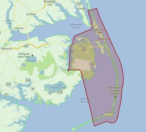
property. Exhibit 1 shows the geographic area of the study, which is Dare County, North

Carolina. Dare County is the easternmost county in North Carolina and boarders on the Atlantic

Ocean. Shoreline erosion has long been measured and recorded in Dare Country along the

entirety of its Atlantic coast. Due to its location and the wealth of historical data on the erosion

rates of the barrier islands, Dare County is uniquely suited for the purposes of our study.

        Transactions records for this study are obtained from the Dare County Tax Office and

include 33,790 residential real estate transactions that occurred in the county from 1996 through

2012. For each transaction we are able to observe the transaction date, price, parcel number, and

permanent mailing address of the purchaser, which allows us to distinguish between local and

nonlocal buyers. Since many of the properties in this area serve as vacation homes, the

                                                 12

permanent mailing address of the purchaser is, in most cases, different from the address of the

property. We categorize buyers into 4 different groups: 1) local buyers, which are defined as

buyers with a permanent address inside North Carolina, 2) buyers from North Carolina’s two

neighboring coastal states – Virginia and South Carolina, 3) buyers from the South and the

Northeast regions, and 4) buyers from all other origins.4 This classification of buyer origin

allows us to not only test for a possible local vs. nonlocal premium, but also to determine

whether the magnitude of the price premium varies with the buyer’s origin. The variability of the

price premium, in turn, sheds light on the role search costs might play in any nonlocal price

premium. Additionally, we collect zip code level data from the Census of Bureau on the median

value of homes near each buyer’s permanent address, as well as the median level of income and

level of education attainment for that zip code.5 These data enable us to determine whether any

relative local versus nonlocal price premium paid is driven by a price anchoring bias, buyers’

financial strength, or buyers’ ability to collect and process information about the market and the

specific property they purchase.

         We then merge the transactions data with a dataset containing physical descriptions of

45,695 unique residential parcels within Dare County. The physical descriptions data are also

from the Dare Country Tax Office and include detailed information on the number of bedrooms

and bathrooms, number of stories, units in the structure, lot size, date of construction, and a

rating of the structure condition (ranging from below average to excellent). We restrict the

merged sample to include only transactions on single-family properties for which the structure

4
  As a robustness check we also classified buyers based on whether their permanent address is located within 100
miles from the Atlantic Ocean in North Carolina, in North Carolina’s neighboring states or in other states. The
results of our analysis using these classifications are similar to the classification described in the text. For brevity,
we omit the results of this robustness classification from the text.
5
  Education and income data is gathered by the American Community Survey and is based on a 5-year estimate. We
define our education variable as the percentage of population above the age of 25 within each zip code with more
than high school education. Income is defined as income per capita.

                                                           13

size, lot size, number of bedrooms and bathrooms, and structure condition are available.

Moreover, because the description of each property’s characteristics and condition are only

available for the most recent transaction, we only include the most recent transaction price for

each property in our analysis. Following the above exclusions, the number of individual

transactions in our final sample is 13,106.6

         We then develop the main variables of interest for this study, the distance to the ocean

and the proximate erosion rate. First, Google Earth is used to identify whether each transacted

property is located either inland (11,071 transactions) or waterfront (2,035 transactions).

         Next, we use Google Earth to measure and record the shortest physical distance (in feet)

of each waterfront property from the water. Given the physical geography of Dare County, some

of the waterfront properties in the sample face the ocean and some face the sound. Soundfront

properties are similar to oceanfront properties in that both enjoy direct water access and

waterfront views. However, soundfront properties are not exposed to anything approaching the

magnitude of the currents or wave action impacting oceanfront beaches. This means that

shoreline erosion is not a significant concern for the buyers of the soundfront properties. Since

shoreline erosion affects only oceanfront properties, the North Carolina Division of Coastal

Management only records erosion rates for shorelines and inlets adjoining the Atlantic Ocean. As

a result, we further classify our sample of waterfront properties as either oceanfront (854

transactions) or soundfront (1,181 transactions).

         Finally, we employ maps from the North Carolina Division of Coastal Management that

detail the long run average annual shoreline erosion rates along the entire North Carolina coast.

6
  The exclusion of all but the last transaction of each property from our analysis is particularly important with our
sample due to the possibility that previous transactions have been associated with a different structure, a structure at
a different condition or even an empty lot. The likelihood of each of these possibilities is especially high given the
abnormal rate of construction, restructuring or renovation in areas that are exposed to destructive events and to rapid
growth, in general.

                                                          14

These maps are constructed using detailed aerial photographs of the entire North Carolina coast

and then overlaid with the erosion-rate data. They are available to the public at no charge. Using

this information, we are able to identify the exact location of each of the 854 oceanfront

properties on the map and record the rate of shoreline erosion at that location for each property.

Appendix A contains two examples of these maps.

        The final compiled dataset includes the property characteristics, proximity to the water,

and information about the quality of the beaches in terms of the estimated erosion rates. To our

knowledge, this dataset is unique in several respects among both the real estate and economics

literatures and enables us to examine the impacts of proximity-to-the-water on property valuation

while also controlling for the risks imposed by shoreline erosion. As a result, we are able to

eliminate some of the noise and biases inherent in previous studies that only consider these

factors in isolation.

        It is important to note that even relatively stable long run average shoreline erosion rates

can deviate abruptly due to sudden shocks from meteorological events. For example, it is

possible for a shoreline that has exhibited a relatively stable long run erosion rate of 4 feet

annually to suddenly experience a loss of 50 or 100 feet of beachfront during a hurricane or

nor’easter. Following such catastrophic events, however, it is common for the affected shoreline

to return to its normal long run erosion rate, albeit from a new location further inland. Therefore,

the potential for extreme storm-driven departures from the long run average erosion rate is

important for prospective homebuyers to consider when purchasing a property located near the

water, even if the home is situated adjacent to a shoreline with a relatively low long run erosion

rate.

                                                15

Table 1 provides a set of descriptive statistics for the final merged dataset. Panel A

includes general statistics, including the share of the transactions where the purchaser is local

(from North Carolina) versus nonlocal. Local purchasers make up approximately 45% of the full

sample, and the nonlocals comprise roughly 55%. For soundfront properties, the share of local

buyers remains similar to their representation across the full sample—at about 47%. However,

the share of local buyers falls to just 19% for the oceanfront properties in the sample. This points

to a strong preference for oceanfront properties by nonlocal buyers. Even so, 82.1% of the

nonlocal purchasers in the dataset bought a property that is neither soundfront nor oceanfront,

compared with 87.7% for local purchasers (as is shown in greater detail in panel C).

        Panel B includes statistics on the characteristics of the homes included in the sample. The

average lot size is 13,591 square feet, and the average home in the sample has 2.9 baths, 3.7

bedrooms, and sold for a nominal price of just over $330,000. Oceanfront properties are located

315 feet from the water on average, while soundfront properties are located much closer to the

water (an average of just 72 feet). The average long run erosion rate for the oceanfront properties

in the sample is 3.2 feet per year.

        Panel C provides descriptive statistics for the buyer characteristics in the sample. The

panel shows that buyers from North Carolina account for 45% of the transactions in the dataset

while 33% of buyers are from the two neighboring coastal states, South Carolina and Virginia.

Of the remaining nonlocal buyers, 9.3% are from the South7, 9.6% from the Northeast, and the

remaining 3% are from the Midwest (1.8%), West (1.0%)8 or outside the United States (0.3%). It

7
  Buyers from Florida, a state that is included in the South region, only represent 0.9% of the transactions.
8
  We employ the Census four region segmentation in order to define the South, Northeast, Midwest and West
regions.

                                                        16

also appears that, on average, nonlocal buyers purchase larger (in terms of number of bedrooms

and bathrooms) and more expensive properties compared with local buyers.9

4.2. Methodology

        In order to examine the effects of shoreline erosion rates on property prices, we employ

several different hedonic model specifications, beginning with a standard hedonic regression:

                            ∑                                               ∑                             (1)

In this equation,               is the natural logarithm of the transaction price of property i at time t;

    are the coefficients of the vector of                 physical property attributes; λ and μ are the

coefficients of the indicator variables Inland and Sound which take the value of 1 when a

property is located either inland or soundfront, respectively, and 0 otherwise (oceanfront is the

omitted variable);       are the coefficients of the          year indicators; and         is the random error

with a mean of 0 and variance σ2. The physical attributes of the properties included in vector X

are Bath, Bed and Story, which represent the number of bathrooms, bedrooms and stories of the

property, respectively; LnLotSize and LnAge are the natural logarithms of the lot size (in square

feet) and age of the house (in years), respectively; Condition takes a value between 1 and 4,

reflecting the overall reported condition of the property (1 – below average, 2 – average, 3 –

above average and 4 – excellent). The primary purpose of the hedonic regression presented in

equation (1) is to confirm whether oceanfront properties sell for a premium compared with

soundfront properties and whether inland properties sell for a discount compared with waterfront

properties.

9
 The averages of the number of bedrooms, bathrooms and price are statistically different at the 1% level when
properties purchased by local and nonlocal buyers are compared.

                                                        17

In order to determine whether buyers are willing to pay a premium for properties located

closer to the water, we estimate the following regression equation for all waterfront properties, as

well as for oceanfront and soundfront properties separately:

                          ∑                            ∑                                     (2)

In this equation, LnDist is the natural logarithm of the property’s distance from the water in feet.

We then introduce the shoreline erosion rate into our analysis in order to examine the

capitalization of erosion risk into property prices. For the sample of oceanfront properties we

estimate the following regression equation:

                          ∑                                           ∑                      (3)

In this model,             is the long run erosion rate (in feet per year) at the proximate location

of property i. Alternatively, we also analyze the data when replacing                and

with the ratio of the distance from the ocean to the proximate erosion rate                    :

                          ∑                                    ∑                             (4)

A negative coefficient of Erosion in equation (3) would indicate that more rapid long run erosion

rates negatively affect property values, and therefore provide support for Hypothesis 1.

Similarly, a positive coefficient for ErosionRatio in equation (4) would suggest that homebuyers

are willing to pay a premium for a waterfront property located further from the ocean relative to

the rate of erosion experienced in that location. This would also provide evidence for the

capitalization of the long run erosion rate into property prices.

       In order to test Hypothesis 2, that the capitalization of the rate of erosion and the distance

of properties from the shore is negligible for properties for which the destructive event is

expected to occur far into the future, we apply equations (3) and (4) on subsets of our data sorted

into terciles by LnDist or ErosionRatio. Coefficients that are increasing in magnitude for the

                                                 18

Erosion or ErosionRatio for properties with lower LnDist or higher ErosionRatio would support

Hypothesis 2. Additionally, we apply equation (2) to oceanfront properties segmented by

differing Erosion thresholds. A larger negative LnDist coefficient for the tercile that includes the

lowest Erosion values would also provide support to Hypothesis 2.

       The existing literature provides evidence that nonlocal buyers purchase properties for a

premium, on average, compared with nonlocal buyers. Lambson, McQueen and Slade (2004)

provide evidence that a price anchoring bias and higher search costs contribute to the relative

price premium. In this paper we revisit the nonlocal premium hypothesis presented by Lambson,

McQueen and Slade.

       We analyze several different specifications of the following regression equation in order

to investigate the nonlocal price premium.

             ∑

                                                             ∑                              (5)

where Local, CoastNeigh and S&NE are dummy variables with a value of 1 if the buyer’s origin

is North Carolina, a neighboring coastal state and the South or the Northeast, respectively, and 0

otherwise. The origin characteristic vector (OriginChar) includes our education measure

(OriginEdu) and the natural log of the per capita income (OriginInc) and median housing value

(OriginVal) at each buyer’s zip code of origin. The coefficients of the location origin variables

indicate whether a nonlocal price premium exists and whether it varies with buyer origin. The

coefficients of OriginEdu, OriginInc and OriginVal variables allow us to examine whether buyer

characteristics like education, income, and home values in the area of origin are correlated with

the transaction price. As a robustness check, we also run regression specification (5) on the top

                                                19

and bottom 50% of the transactions in terms of price for inland, soundfront and oceanfront

properties. This price segmentation addresses the fact that nonlocal buyers, on average, purchase

more expensive homes compared with local buyers.

         To examine the effect of short-term shocks to the erosion rate on the capitalization of

erosion risk into property values, we identify periods following hurricanes that caused severe

damage to the area. According to the National Oceanic and Atmospheric Administration

(NOAA), 70 named storms (hurricanes or tropical storms) affected the eastern part of North

Carolina during the 1995 to 2012 time period, with differing levels of severity. Fortunately, most

of these events were associated with only minor physical destruction and had minimal lasting

effects on the area. However, three storms: Hurricane Fran (September1996)10, Hurricane Floyd

(September 1999)11 and Hurricane Isabel (September 2003)12 were particularly destructive to the

area, with physical damages exceeding $500 million13 in addition to the loss of human lives.

         We create three indicator variables (Yhit) that include the two-year period14 immediately

following each of these three catastrophic events. These indicator variables are then interacted

with Inland, Sound, LnDist and ErosionRatio variables as follows:

                               ∑                                                 ∑

         ∑                                                                                                   (6a)

10
    The physical damage from Hurricane Fran was reported to be $2.55B in 1996. Hurricane Fran was also
responsible for 14 deaths of which 6 were classified as direct deaths. At the time, this hurricane was considered to be
the state’s worst natural economic disaster.
11
   The physical damage from Hurricane Floyd was reported to be $3.7B in 2007. Hurricane Floyd was also
responsible for 35 direct and 16 indirect deaths. Floyd compounded the effect of Hurricane Dennis for which severe
beach erosion was reported and occurred only a few weeks prior to Floyd. North Carolina Governor Jim Hunt
described the hurricane as "the worst disaster to hit North Carolina in modern times."
12
   The physical damage from Hurricane Isabel was reported to be $450M in 2003. Most of the damage from this
hurricane was concentrated in Dare County where thousands of homes washed away. The storm surge produced a
wide inlet (up to 2,000 feet) that isolated some roads in the area for up to two months.
13
   2013 dollars.
14
   We also experimented with “post” periods that include the one-year and three-year periods that immediately
followed each of our three identified catastrophic events. Results from these analyses are similar to the two year post
windows and therefore omitted in the interest of brevity.

                                                          20

∑                                       ∑

       ∑                                                                                   (6b)

                           ∑                                           ∑

       ∑                                                                                   (6c)

                           ∑                                  ∑

       ∑                                                                                   (6d)

Consistent signs across the coefficients for τ1, τ2, τ3 and τ4 for the three post periods would

provide support for Hypothesis 3, indicating buyers temporarily adjust the risk premium during

post catastrophic-event periods for properties that are waterfront, closer to the shore, and with

lower ratios of distance-to-erosion rate.

       For robustness, we also apply equations (3) and (4) to examine the capitalization of land

erosion for subsamples of the data. These robustness checks allow us to observe whether the

capitalization of erosion risk into property prices varies by specific time period or housing price

trend. Therefore, we segment our dataset two ways. The first segmentation separates the full

dataset into observations occurring during the early period of our study (1996-2003) and those

occurring in the late period of our study (2004-2012). The second segmentation divides the data

into three periods of differing housing price trends: Boom, bust, and normal. We define the

period between 1996 and 2002 as normal in terms of price appreciation, the period from 2003 to

2006 as the boom period, and 2007 through 2012 as the bust period.

                                                21

5. Results

5.1. Capitalization of Land Erosion into Property Prices

       Table 2 displays the results of the hedonic regressions from equations (1) through (4).

The adjusted R-squares of these regressions range from 60% to 67% and the signs of the

regression coefficients are generally in line with expectations. The coefficients for housing

characteristic variables such as the number of bathrooms (Bath), number of bedrooms (Bed),

numbers of stories (Story), lot size (LnLotSize), and property condition (Condition) are all

positive and statistically significant, which is consistent with the findings of numerous other

studies. However, the coefficient of the property’s age variable (LnAge), which is expected to be

negative, is instead positive and significant. While it is not easily verifiable from our data,

conversations with real estate agents from the area reveal that the most desirable locations along

the coast were developed first, and the newer homes have been generally built on less desirable

lots. Additionally, the agents indicate that the overall quality of craftsmanship and finishes in

older homes often surpasses those of newer homes.

       As expected, the results from the hedonic regression defined in equation (1)

(specification 1) reveal that oceanfront properties (the omitted variable in the model) sell for a

premium to soundfront properties, which in turn sell for a premium compared with inland

properties. Specifications (2), (3) and (4) of Table 2 report the results of the hedonic regression

defined in equation (2). Specification (2) refers to all waterfront properties (oceanfront and

soundfront combined) and specifications (3) and (4) refer separately to soundfront and

oceanfront properties, respectively. In all three specifications the coefficient of the distance from

the property to the water (LnDist) is negative and statistically significant, suggesting that when

shoreline erosion rates are not explicitly considered, homebuyers are willing to pay a premium

                                                 22

for properties which are closer to the water. These results conflict with some previous studies

(Gopalakrishnan, Smith, Slott and Murray 2010; Landry, Keeler and Kriesel 2003; Pompe and

Rinehart 1995), which provide evidence for buyers’ willingness to pay extra for an additional

foot of sand. However, these studies did not control for the long run erosion rate and therefore

were unable to isolate the desire to be closer to the water from the desire to be protected from the

risk of shoreline erosion.

       Specifications (5) and (6) present the results of two different hedonic regressions from

equation (3). Specification (5) shows a negative and statistically significant coefficient for the

long run erosion rate variable (Erosion). The magnitude of the negative coefficient becomes even

larger when the property’s distance from the water is considered (specification 6). It is important

to note that in this specification, the magnitude of the LnDist coefficient is roughly double that

found when erosion is not included in the regression (specification 4). This is consistent with the

notion that once the erosion rate factor is considered, buyers prefer to be closer to the water. The

results presented in specifications (5) and (6) clearly suggest that homeowners consider the land

erosion factor when purchasing a home and discount housing located in more rapidly eroding

areas. In other words, it seems clear that long run erosion risk is capitalized into residential

property prices, in support of Hypothesis 1. The final specification (7) in Table 2 reports the

results from the hedonic regression defined in equation (4). The positive and statistically

significant coefficient of the ErosionRatio variable illustrates the tradeoff between the desire to

be located closer to the ocean and the consideration of the long run land erosion rate. The fact

that home buyers are willing to pay a premium for an oceanfront property with a high distance-

to-erosion ratio also confirms the results from specifications (5) and (6). Overall, Table 2

resolves some of the inconsistencies in the existing literature regarding the impact of beach width

                                                23

on property prices. The results highlight the fact that being closer to the ocean commands a

premium, but that erosion rate must also be considered.

       Table 3 provides a closer look at how long run erosion rates are capitalized into the prices

of residential real estate. Specifications (A1), (A2) and (A3) employ the hedonic regression from

equation (3) on terciles of the oceanfront properties in the dataset sorted by distance from the

water. Specification (A1) refers to the one-third of oceanfront properties closest to the water.

Specifications (A2) and (A3) include the middle and most distant thirds of the oceanfront

sample, respectively. The results in these three specifications suggest that the long run erosion

rate is capitalized to the greatest extent into the prices of properties located closest to the ocean

(A1). The capitalization of the erosion rate is slightly smaller for properties in the middle tercile

in terms of distance from the ocean (A2) and becomes statistically insignificant for properties in

the most distant tercile (A3).

       Specifications (B1), (B2) and (B3) employ the hedonic regression from equation (4) on

terciles of the oceanfront data sorted by the distance-to-erosion ratio (ErosionRatio). Similar to

the segmentation methodology for physical distance from the ocean, specification (B1) includes

the tercile of properties with the lowest distance-to-erosion ratio, while specifications (B2) and

(B3) contain the middle and the highest distance-to-erosion terciles, respectively. Consistent with

the findings presented in specifications (A1) through (A3), although to an even greater extent,

the ratio of distance from the ocean to the long run erosion rate appears to only be capitalized for

properties in the lowest distance-to-erosion ratio tercile (specification B1). For the other two

terciles the coefficients of distance-to-erosion ratio are statistically insignificant. Again, this

implies that home buyers do not factor shoreline erosion rates into their reservation price unless

the erosion risk to the subject property is high.

                                                    24

Finally, specifications (C1) and (C2) examine the capitalization of land erosion into

property prices among different ranges of long run erosion. Specification (C1) includes all

properties located in areas with long run annual erosion rates below 2.5 feet, and specification

(C2) includes all properties associated with long run annual erosion rates of 2.5 feet and greater.

We find the coefficient of the LnDist variable is only negative and statistically significant for

properties located in low erosion rate areas (C1) and statistically insignificant for properties

located in high erosion rate areas (C2). This indicates that proximity to the ocean only commands

a premium for properties located in areas with low erosion rates and further supports the results

from specifications (A) and (B).

       Overall, the findings presented in Table 3 support Hypothesis 2 and suggest that

homebuyers generally ignore the risk of shoreline erosion unless it appears to be a near-term

threat. In other words, oceanfront homebuyers are willing to pay a premium for closer proximity

to the water and do not factor erosion risk into the purchase price unless the property is either

very close to an eroding beach and/or located in a rapidly eroding area.

5.2. Buyers’ Origin

       The results reported in Panel A of Table 4 shed light on the extent to which nonlocal

buyers pay a premium for properties compared to local buyers. The existing literature interprets a

price premium paid by nonlocal buyers as a market inefficiency and provides some evidence that

the premium is driven by a price anchoring bias and higher search costs.

       Specifications (1) and (2) present the results of the hedonic regression from equation (5)

applied to the full sample with one and three location dummies, respectively. The negative

coefficient of the Local dummy variable in each of the regressions indicates that nonlocal buyers

                                                25

pay a premium when they purchase a property compared with local buyers. The coefficients of

CoastNeigh and S&NE variables are also negative, but smaller in magnitude than the Local

coefficient and the S&NE coefficient is insignificant. This suggests that the premium paid by

nonlocal buyers is positively correlated with the distance of buyers’ origin from North Carolina.

Specifically, North Carolina residents pay the smallest premium, while buyers from the

neighboring coastal states, the South, Northeast, and all other areas (Midwest, West and foreign

countries) pay an increasingly higher premium.15 Assuming that search costs are correlated with

the buyer’s physical distance from the subject property, our results are consistent with the

conclusion of Lambson, McQueen and Slade (2004) that higher search costs contribute to the

nonlocal premium.

         Specifications (3) through (5) repeat specification (2) for inland, oceanfront and

soundfront properties. Generally, the results of these regressions are similar to the results

generated from the full sample, suggesting that the nonlocal premium is not driven by a specific

property type. We noted earlier that nonlocal buyers tend to purchase, on average, larger and

more expensive properties compared with local buyers. Therefore, in specifications (6) and (7)

we repeat specification (2) for the bottom and top 50% of the transactions in terms of the sale

price in each of the inland, oceanfront and soundfront categories. Once again, the results are

similar to those from the full sample, indicating that the nonlocal premium is present across

varying price points and is therefore not driven by the tendency of nonlocal buyers to purchase

higher-priced homes.

15
  We thank an anonymous referee for suggesting the examination of North Carolina homestead exemption as a
possible driver for the nonlocal premium. While the state of North Carolina offers homestead exemption, these
exceptions are only available to the elderly, disabled and as a low income families. Given that these exemptions only
capture the weakest economic segments of the population, it is reasonable to assume that due to high property prices
of our subject area, the vast majority of buyers would not qualify for these exemptions.

                                                         26

Panel B of Table 4 presents results from regressions that employ the zip code

characteristics of the buyer’s origin. The results from specifications (1) through (3) show that,

considered independently, the level of education (OriginEdu), housing valuation (OriginVal) and

income per capita (OriginInc) at the buyer’s origin are all positively related to the price a buyer

pays for a property. These results are not surprising given the positive correlation between the

three characteristics. However, when these characteristics enter the regression simultaneously in

specification (4), the coefficients of OriginVal and OriginInc remain positive and statistically

significant while the coefficient of OriginEdu becomes negative and statistically significant. This

suggests that buyers with higher income levels and from areas where housing is more expensive

tend to pay more for properties, while more educated buyers tend to pay less, on average. The

positive coefficient of the OriginVal variable is consistent with the price anchoring bias

hypothesis of Lambson, McQueen and Slade (2004). The negative coefficient of the OriginEdu

variable suggest that, on average, more sophisticated buyers are able to purchase properties at a

relative discount. When local and nonlocal buyers are examined separately in specifications (5)

and (6), the coefficient of OriginEdu is no longer statistically significant and the sign switches to

positive in the case of nonlocal buyers (specification 6). Of the three origin characteristics, only

the coefficient of OriginVal retains its sign (positive) and significance for local buyers

(specification 5), while the coefficient of OriginInc is the only coefficient that retains its sign

(positive) and significance for nonlocal buyers (specification 6). These results suggest that the

buyer’s income is the primary driver of the nonlocal price premium and therefore contradicts the

notion of a price anchoring bias. Also, the insignificant coefficients of the OriginEdu variable

weakens our previous finding on the relation between buyers’ level of sophistication and relative

price discounts.

                                                 27

5.3. Long Run Erosion Rate Shocks

         Table 5 presents the results of our analysis of the effect of shocks to the long term erosion

rate on the capitalization of erosion risk into property prices. As per the hedonic regressions from

equations (6a) through (6d) we interact the post hurricane periods with four different variables.

Generally, the results presented in Table 5 provide little evidence that shoreline erosion risk is

capitalized differently during post-hurricane periods. The results from equation (6a)

(Specification 1) indicate that inland properties sold for a relative premium following hurricane

Fran (S1), but for a relative discount following hurricane Floyd (S2). Specification (2) shows no

clear relative discount or premium for soundfront properties following the three catastrophic

events. Finally, Specifications (3) and (4) indicate that oceanfront properties located a greater

distance from the ocean, or with a higher ratio of distance to erosion rate, sold for a premium

following hurricane Isabel (S3), but show no sign of a premium following hurricanes Fran and

Floyd.

         It is possible that these weak and variable results are due to the high frequency of named

and unnamed storms (including nor’easters which, although unnamed, can be extremely severe)

that impact the area during the sample period. While most of these storms did not have a lasting

impact on properties located in Dare County, the high frequency of storms impacting the area

makes disentangling severe post-catastrophic events from less severe events a significant

challenge. Therefore, we believe the results presented in Table 5 are generally in line with

Hypothesis 4.

                                                  28

5.4. Robustness Checks

       As a robustness check we examine whether the evidence of capitalization of the erosion

rate into property prices is triggered by a specific time period or market price trend. As we

describe in the methodology section, we first divide the dataset into two segments, which include

the observations that took place during the early period of our study (1996-2003) and the late

period of our study (2004-2012). We then repeat the regression analyses presented in Table (2)

for both time periods. The results of this analysis reveal that the capitalization of shoreline

erosion into property prices during the earlier and the later time period is similar and therefore

suggests that the general findings presented in this paper persist throughout the entire sample

period. For the sake of brevity, these results are not tabulated.

       We continue by analyzing segments of the data based on different housing price trends.

The normal price trend segment includes the 1996 through 2002 time period, the boom period is

defined as occurring between 2003 and 2006, and the bust period includes all transactions that

took place between 2007 and 2012. Once again, we repeat the regression analyses presented in

Table 2 for each of these three time periods. The regression results for each of the segmented

periods are not materially different from the results presented in Table 2 and thus suggest our

general findings are not being driven by a particular housing price trend. For brevity, these

results are also not presented.

6. Conclusion

       This paper explores how the risk associated with shoreline erosion is capitalized into

residential real estate prices. The results of our analysis show that while oceanfront properties

command a higher premium when located closer to ocean, the rate of erosion at the property

                                                  29