Semi-supervised Multi-task Network For Image Aesthetic Assessment
←
→
Page content transcription
If your browser does not render page correctly, please read the page content below
https://doi.org/10.2352/ISSN.2470-1173.2020.8.IMAWM-188
                                                                                            © 2020, Society for Imaging Science and Technology

Semi-supervised Multi-task Network For Image Aesthetic
Assessment∗
Xiaoyu Xianga , Yang Chenga , Jianhang Chena , Qian Linb , Jan Allebacha
a School of Electrical and Computer Engineering, Purdue University, West Lafayette, IN 47907, USA
b HP Labs. Palo Alto, CA 94304, USA

Abstract                                                                 factors in a given image: the theme, or semantic elements within
      Image aesthetic assessment has always been regarded as a           the image, and the proper style and composition, such as the rule
challenging task because of the variability of subjective prefer-        of thirds, shallow DOF (depth of field), etc. In other words, the
ence. Besides, the assessment of a photo is also related to its style,   aesthetics of an image is assessed through a complex interplay be-
semantic content, etc. Conventionally, the estimations of aesthetic      tween themes and styles. Moreover, images with obvious styles
score and style for an image are treated as separate problems. In        are usually linked to high aesthetic appeal.
this paper, we explore the inter-relatedness between the aesthetics            Inspired by the intrinsic connection between style and aes-
and image style, and design a neural network that can jointly cat-       thetic assessment, this work entangles these two problems to-
egorize image by styles and give an aesthetic score distribution.        gether by a multi-task network (MTNet), that can be trained to
      To this end, we propose a multi-task network (MTNet) with          encode given images into feature vectors and predict aesthetic
an aesthetic column serving as a score predictor and a style col-        scores, as well as the style category, where the feature vectors
umn serving as a style classifier. The angular-softmax loss is ap-       are shared by an aesthetic column and a style column. For effi-
plied in training primary style classifiers to maximize the margin       cient training, we first pre-train the encoder on the AVA training
among classes in single-label training data; the semi-supervised         set with A-softmax loss [16], and iteratively fine-tune it by a self-
method is applied to improve the network’s generalization ability        training approach. The acquired encoder serves as a backbone for
iteratively. We combine the regression loss and classification loss      MTNet. Overall, the proposed MTNet is shown to improve the
in training aesthetic score. Experiments on the AVA dataset show         performance over the previous state-of-the-art architectures.
the superiority of our network in both image attributes classifica-
tion and aesthetic ranking tasks.                                        Related Works
                                                                         Aesthetic score prediction
Introduction                                                                   Deng et al [4] summarizes early works using hand-crafted
     Image aesthetic assessment is essential to smart photo album        aesthetic-rule based features to design an assessment method [3,
applications, such as the criteria for image retrieval systems and       15, 25]. More recent studies show that using a deep feature repre-
cover photo recommendation. Besides, it can serve as a guide             sentation method boosted by large-scale datasets performed much
for image enhancement. For a long time, image aesthetic assess-          better than traditional hand-crafted features [10]. The training
ment has been regarded as a branch of image quality assessment,          data are often collected from online photography communities,
which includes the estimation of several image quality attributes,       where people rate each photo by integer scores from 1 to 10. By
such as sharpness, noise, artifacts, etc. While the goal of image        weighted averaging all scores, it should be possible to get the final
quality assessment algorithms is to be consistent with the quality       score for an image. Higher scores represent a positive assessment
assessment of a human viewer [23], image aesthetics cannot be            from most of the people. Based on the score, one can compare two
fully represented by image quality alone. Sometimes the human            images in terms of their aesthetic aspects, and classify an image
assessment of aesthetics even contradicts the assessment of qual-        into a high or low aesthetic category.
ity for the same image. Compared with other computer vision                    Some researchers [27] choose to represent image aesthetic
problems, image aesthetic assessment is even more challenging            quality with the score, either in numerical encoding or binary en-
because of its subjective nature [26], which means we can hardly         coding. However, other researchers propose that due to the sub-
find a universal rule to judge a given image.                            jective nature of human annotators, the score distribution can be
     In recent years, convolutional neural networks have been            really diverse. Especially, the mean score is easily influenced by
widely applied in image aesthetics prediction [2, 7, 9, 10, 14,          low and high extremes from minor annotators. Besides, previous
21, 24, 27] thanks to the publishing of large-scale datasets, such       papers [9, 10, 11] also notice that the distribution of mean score
as AVA [22], AADB [13], and IDEA [11]. These datasets are                or the number of the votes for each image is far from evenly dis-
composed of image data and meta-data, such as crowd-sourcing             tributed as shown in Figure 1. In order to solve this problem, more
scores, semantic categories, and style or attributes. For human          recent works propose to use the score distribution in image aes-
viewers, although there is no strict rule that directly corresponds      thetic assessment. The progress on this path is mainly to use more
to aesthetic scores, they are perceptually influenced by following       and more appropriate loss functions to make the network’s output
                                                                         approach the target distribution. Jin et al [9] applies the weighted
    ∗ Research   supported by HP Inc., Palo Alto, CA.                    Chi-square distance loss to predict the average score and standard

IS&T International Symposium on Electronic Imaging 2020
Imaging and Multimedia Analytics in a Web and Mobile World                                                                                 188-1
deviation from the rankings distribution. Wang et al uses asym-              lated as follows:
metrical Kullback-Leibler (KL) divergence as the loss function
and processes the AVA dataset’s score distribution into a Gaussian                                      1   N
                                                                                                                        ezyi
                                                                                  Lso f tmax = −            ∑ log ∑C         zj
                                                                                                                                               (1)
distribution to train their DBN network. Hou et al [8] and Talebi                                       N   i=1         j=1 e
et al [24] uses squared EMD (earth mover’s distance) loss [8]
to train a CNN to predict the score histogram. Murray et al [21]                  where N is the number of training samples, C stands for the
employs the Huber loss, which is more robust to outliers, in their           number of classes. z j is the activation of the j−th neuron in a
APM network. Cui et al [2] applies the traditional label distri-             fully connected layer with corresponding weight vector W j and
bution learning method to predict an aesthetic score histogram.              bias b j . Each neuron is supposed to predict the score z j for target
Jin et al [10] compares previously proposed loss functions and               class j. Softmax loss is based on the Euclidean margin of differ-
chooses the cumulative Jensen-Shannon divergence.                            ent classes. If we fix the bias b j = 0 and express x in the polar
                                                                             coordinate system, the predicted score z j can be written as:

                                                                                  z j = W jT x = ||W j || · ||x|| cos θ j                      (2)

                                                                             where θ j denotes the angle between W j and the input x. Previous
                                                                             papers [6, 16] use a simplified example of binary classification to
                                                                             illustrate the idea of A-softmax. According to Equation 2, three
                                                                             components can influence the predicted score: an embedding fea-
                                                                             ture vector x, and the learned weights W1 and W2 , which represent
                                                                             the class centers. For this binary classification problem, the deci-
                (a)                                  (b)
Figure 1.   The score and vote number distribution of the AVA dataset: (a)   sion boundary is:
The distribution of the number of votes per image; (b) The distribution of
                                                                                  ||W1 || cos θ1 = ||W2 || cos θ2                              (3)
mean score per image.

                                                                                  For a single label problem, a sample is classified into the
                                                                             class j that has a higher score z j . As shown in Equation 3, the
Image style classification                                                   decision boundary depends on both the norm and angle of the
                                                                             classification center. Even if the angles between a feature vector
      Early works [5] use hand-crafted features to describe photo
                                                                             and two class centers are the same, it tends to be categorized to
styles. Lu et al [17] utilizes style attributes of the image to help
                                                                             the class with a larger L2 norm. Besides, a feature vector with a
improve the aesthetic classification accuracy, where the style-
                                                                             larger L2 norm would output a higher prediction score.
SCNN is pretrained on the AVA dataset and its output is concate-
                                                                                  In this paper, we want to eliminate the influence of norms
nated to predict the binary categorization result. Inspired by the
                                                                             and classify over angularly discriminative features (The reason
multi-column and concatenation methods, Kong et al [13] incor-
                                                                             to disentangle the L2 norm is illustrated in the Appendix). We
porates joint learning of photographic attributes and image con-
                                                                             normalize ||W j || and ||x|| to 1 as follows:
tent to predict image aesthetic scores.
                                                                                           W j∗                     x∗
Embedding of the MTNet                                                            Wj =              ,       x=                                 (4)
                                                                                          ||W j∗ ||               ||x∗ ||
Network Architecture
                                                                             where W j∗ and x denote the original weight and feature vectors.
     The architecture of MTNet is shown in Figure 2. It can be               After normalization, only the angles between the feature vector
generally divided into two parts: an image encoder, and a multi-             and the two weight vectors are relevant to the decision boundary:
column network to realize specific tasks, including an aesthetic
column that outputs the score distribution for the image’s aesthet-               cos θ1 = cos θ2                                              (5)
ics, and an attribute column that classifies the attributes of the
given image. The image encoder roughly follows the same struc-                    That is, the sample tends to be classified into the class j that
ture as SphereFace [16], which is a modified ResNet. Input im-               has larger cos θ j , which corresponds to a smaller angle. We can
ages are encoded into a 512-dimension feature vector for further             regard the normalization as mapping the weight vector and feature
processing in multi-column networks.                                         vector to a unit hypersphere. As analyzed above, ||W j || = 1, ∀ j
                                                                             and ||x|| = 1. The modified A-softmax is:
      The attribute column is composed of a fully connected layer
that converts the 512 × 1 feature vector into a 14-class prediction
                                                                                               1    N
                                                                                                                   em cos θyi
result. Since we apply angular-softmax (A-softmax) to train the                   Lang = −         ∑ log ∑C             m cos θ j
                                                                                                                                               (6)
                                                                                               N                  j=1 e
classifier, the predicted score for each class ranges from −1 to 1.                                i=1

                                                                             where m is the scale factor that controls the size of the margin.
Angular-softmax                                                              From softmax to A-softmax loss, our network learns image fea-
     A-softmax loss is a novel loss function modified from soft-             tures with an angular margin. A-softmax has already demon-
max loss, first proposed by [16]. Traditional softmax loss is com-           strated its superiority in many tasks including face recognition
monly used for classification tasks. For an input feature vector xi          and verification [16], person re-identification [6], and other gen-
and its corresponding label yi , the softmax function can be formu-          eral classification tasks [28].

                                                                                              IS&T International Symposium on Electronic Imaging 2020
188-2                                                                                   Imaging and Multimedia Analytics in a Web and Mobile World
Figure 2. Structure of the MTNet.

Semi-supervised Training
      In most computer vision research, data augmentation in-
cluding random cropping, re-centering, RGB normalization, and
noise-injection is used as an effective tool to improve the net-
work’s robustness. However, cropping and re-centering would
change the composition of an image. This would lead to to-
tally different aesthetic rankings for human perception. And RGB
normalization would make the acquired network less sensitive to
brightness, white balance, etc, which happen to be important fac-
tors for image aesthetic assessment. Thus, methods of data aug-
mentation should be carefully chosen for image aesthetic related
research projects. In this paper, we horizontally flipped 50% of         Figure 3. The diagram of the iterative learning process.
training images to ensure the least influence on the data’s inner
consistency. All images are resized to 112 × 96 to satisfy the re-
quirements of the network input.                                         Combining the Regression and the Classification
      In the AVA attributes subset, all training images have a sin-            The target output of the aesthetic column is the score his-
gle label, while the number of labels of test images can vary from       togram as mentioned in the earlier introduction of the AVA
zero to many. The difference between the training and testing            dataset. On the one hand, the aesthetic score prediction task
data requires our network to have the ability to generalize, while       is firstly a regression problem that aims to approach the target
maintaining discrimination between multiple attribute classes. A         score as closely as possible. The mean square error (MSE) loss
semi-supervised strategy is used to achieve this goal. First, we         is widely adopted for solving such regression tasks. On the other
train the primary classifier with A-softmax loss until it actually       hand, the predicted scores serve as a reference for binary clas-
learns discriminative attribute features (reaching 99.9823% accu-        sification, that categorizes the input image into either “good” or
racy on the training set in our experiment). Then we apply this          “bad” categories. Cross entropy loss, softmax loss, etc. are used
pre-trained classifier on training data again to predict the attribute   to solve this classification problem.
scores for each image. With the reference of ground truth, we add              In this paper, we combine the regression problem with the
the attribute classes for which the prediction scores are higher         classification problem to get better results. By adding extra lay-
than a certain threshold into the training labels. After scanning        ers to the aesthetic column, our network is capable of outputting
the whole dataset, we get a new training set with multi-label at-        a score histogram and binary classification scores. For these two
tributes. Then, we re-train the classifier with the acquired labels      types of outputs, we apply the MSE loss and the Cross-Entropy
and re-apply it to the training set again to propose new attribute la-   loss, respectively, to the two tasks. The advantage of combining
bels to training images. We repeat this process until the classifier     the two losses is to increase distinctions among training data. As
stops changing. The iterative learning algorithm is summarized in        shown in Figure 1, the score histogram of the AVA dataset is not
Figure 3.                                                                evenly distributed. Previous research [11] has declared that he un-
      After the iterative learning process, we are supposed to have      balanced training set makes the training of neural networks easy
a robust classifier that can distinguish image styles. This classifier   to over-fit. The adding of classification loss teaches the network
can be divided into an image encoder and an attribute column. As-        to be more discriminative on the images near the threshold.
suming that the encoded feature vectors have enough information
reflecting image attributes, it is reasonable to expect that informa-    Experiments
tion about aesthetic scores is also included in the latent features.           In training the attribute classifier, we choose m = 4. Stochas-
The following section introduces how to train an aesthetic column        tic gradient descent is used as the optimizer, with a momentum of
based on this assumption.                                                0.9 and a weight decay of 0.0005. We fix the parameters of the

IS&T International Symposium on Electronic Imaging 2020
Imaging and Multimedia Analytics in a Web and Mobile World                                                                                 188-3
outputs. In our experiment, the distance thresholding method out-
performs the direct output of the fully-connected layer by 0.05%.
Aesthetic Score Histogram Prediction
Table 2 shows the comparison of score histogram predic-
tion results on AVA dataset. The divergence between the pre-
dicted histogram and the ground truth is measured by several
metrics: PED (the Euclidean distance between two probability
distribution functions); PCE (cross-entropy between two prob-
ability distribution functions); PJS (the symmetrical version of
the Jensen-Shannon divergence between two probability distribu-
tion functions); PCS (Chi-square distance between two probabil-
ity distribution functions) [9]; PKL (the symmetrical version of
Kullback-Leibler divergence between two probability distribution
function) [26]; CED (Euclidean distance between two cumulative
distribution functions) [8, 27]; and CJS (the symmetrical version
of the Jensen-Shannon divergence between two cumulative dis-
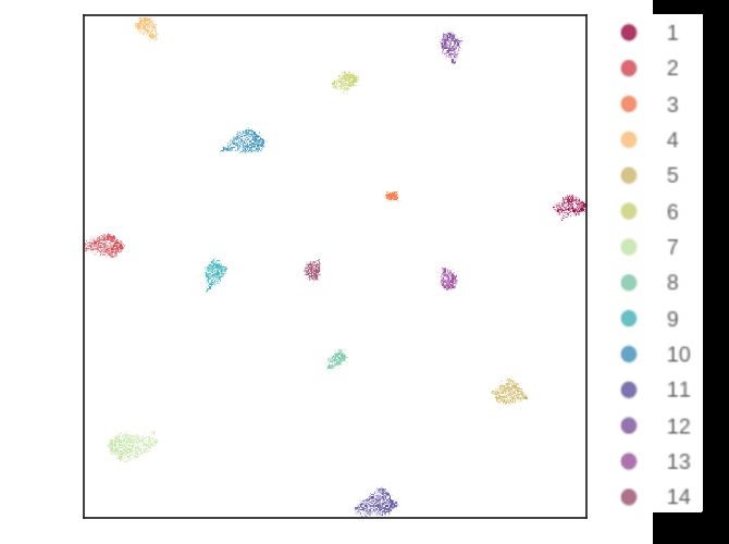
Figure 4. The attributes of photos in the AVA datasets embedded into two tribution functions) [10]. With the exception of PCS, our result
dimensions by the UMAP. outperforms the previous best ones by a large margin.
Conclusion
image encoder when training the aesthetic column, and fine-tune In this paper, we present a multi-task deep convolutional neu-
the remaining layers with AVA’s training set. During the fine- ral network for image aesthetic quality assessment and style cate-
tuning, the optimizer’s weight decay is changed to 0.005 while gorization. Rather than solving these problems with two separate
others remain the same. models, in our MTNet the aesthetic column and the style column
We perform two types of evaluation: the classification accu- share the same image encoder trained by a semi-supervised ap-
racy using the benchmark-setting on AVA style experiments [22], proach, which provides a new insight for solving the multi-label
and divergence between the predicted score histogram and the classification problem with single-label data. Besides, we intro-
ground truth in AVA aesthetic image lists [22] using the same met- duce A-softmax loss in the image aesthetics area for the first time,
rics as described in [10]. and demonstrate its effectiveness on style classification in an an-
gular hyperspace. Our experiment results prove that the perfor-
Style Classification mance of aesthetic assessment can be leveraged by style classifi-
To prove that our image encoder actually learns the features cation. The evaluation results on the AVA dataset show that our
representing image attributes and scores, we visualize the encoded approach outperforms earlier-reported methods for the six out of
features by dimension reduction using UMAP (Uniform Manifold the seven metrics evaluated.
Approximation and Projection) [19, 20], as shown in Figure 4.
For simplicity, we plot the AVA attribute training set where each Appendix
image only corresponds to one label. We can see that the attributes Interpretation of L2 Norm
of different labels form separate clusters in the hyperspace, which To understand what the L2 norm of feature vectors encoded
indicates our network is able to learn a discriminative embedding by our network represents, we select the top three and bottom
of the latent features of the AVA images. three pictures of each style according to their feature vectors’ L2
We compare our model’s performance on the test set of AVA, norm. The selected pictures are shown in Figure 5.
where each image may correspond to 0 to n labels. Following The feature vector is a distilled representation of the original
the approach taken in previous papers, we report AP (Average image. In our work, the network basically serves as a discrimina-
Precision), which computes the average precision value for recall tor for good images with recognizable styles. Each dimension of
values over 0 to 1, and mAP (mean Average Precision), which is the vector represents a detectable feature related to the network’s
the average AP for all categories. purpose, which implies that a higher norm corresponds to stronger
Table 1 shows that our method achieves the second-best re- detectable features in the image. The pictures in Figure 5 sup-
sults for style classification. Here, we list our results acquired port this: images with higher norms usually have richer content
from three different methods: 1) primary method, which is the pri- and more distinguishable features. In order to get rid of the bias
mary classifier that is trained on the original single-label dataset; caused by these factors of the L2 norm for style classification, we
2) iterative learning model, which is acquired based on the pri- chose A-softmax loss along with cosine distance as a comparison
mary classifier through the iterative learning process as men- metric.
tioned previously; 3) nearest cluster method. It uses the model
trained from iterative learning. But instead of taking the classifi- References
cation output from the last fully connected layer, it takes the 512- [1] Karsten M Borgwardt, Arthur Gretton, Malte J Rasch, Hans-Peter
dimension feature vector to compute the cosine distance to the Kriegel, Bernhard Schölkopf, and Alex J Smola. Integrating struc-
class’s average centers of each style category. The classes with tured biological data by kernel maximum mean discrepancy. Bioin-
a distance that is lower than the threshold are taken as prediction formatics, 22(14):e49–e57, 2006.
IS&T International Symposium on Electronic Imaging 2020
188-4 Imaging and Multimedia Analytics in a Web and Mobile World
Method                           AP (Average Precision)    mAP (mean Average Precision)
                        Murray et al [22]                         n/a                       53.85%
                        Karayev et al[12]                         n/a                        58.1%
                        Lu et al[17]                            56.93%                      56.81%
                        DMA-Net [18]                            69.78%                      64.07%
                        Kong et al[13]                          59.11%                      58.73%
                        Ours (primary)                          60.75%                      58.89%
                        Ours (iterative learning)               61.19%                      59.47%
                        Ours (class distance)                   62.03%                      60.28%

Table 1: Image style classification results on the AVA testet. Bold font indicates the best result, and underline font indicates the
second-best result.
                              Method                PED        PCE      PJS    PCS      PKL    CED      CJS
                              PED                   0.197      2.830   0.059   0.105   0.728   0.323   0.068
                              RS-PED                0.189      2.733   0.055   0.094   0.657   0.324   0.067
                              PCE                   0.167      2.773   0.041   0.075   0.442   0.279   0.049
                              RS-PCE                0.169      2.771   0.046   0.071   0.438   0.279   0.047
                              PJS                   0.185      2.828   0.051   0.093   0.527   0.326   0.053
                              RS-PJS                0.183      2.776   0.049   0.091   0.523   0.327   0.049
                              PCS[9]                0.182      2.807   0.045   0.082   0.450   0.287   0.045
                              RS-PCS                0.175      2.783   0.045   0.079   0.423   0.277   0.044
                              PKL[26]               0.163      2.779   0.039   0.073   0.389   0.270   0.044
                              RS-PKL                0.164      2.778   0.037   0.071   0.386   0.268   0.043
                              MMD[1]                0.201      2.831   0.064   0.112   0.710   0.339   0.068
                              RS-MMD                0.196      2.824   0.063   0.097   0.710   0.322   0.054
                              Huber[21]             0.184      2.775   0.044   0.078   0.409   0.279   0.053
                              RS-Huber              0.183      2.774   0.045   0.074   0.402   0.271   0.048
                              CED[8][27]            0.182      2.799   0.047   0.085   0.502   0.294   0.049
                              RS-CED                0.180      2.792   0.048   0.082   0.502   0.283   0.047
                              CJS[10]               0.163      2.779   0.039   0.072   0.382   0.266   0.041
                              RS-CJS[10]            0.158      2.760   0.037   0.068   0.381   0.260   0.040
                              LDL Method[2]         0.303        -       -       -       -       -       -
                              Ours                  0.060      2.218   0.009   0.081   0.018   0.110   0.012

Table2: Comparison of score histogram prediction errors on the AVA dataset. Smaller numbers indicate better results. The results
are obtained by training with different loss functions as mentioned in [10]. Bold font indicates the best result.

Figure 5. Images selected by feature vectors’ norm for each style

IS&T International Symposium on Electronic Imaging 2020
Imaging and Multimedia Analytics in a Web and Mobile World                                                                        188-5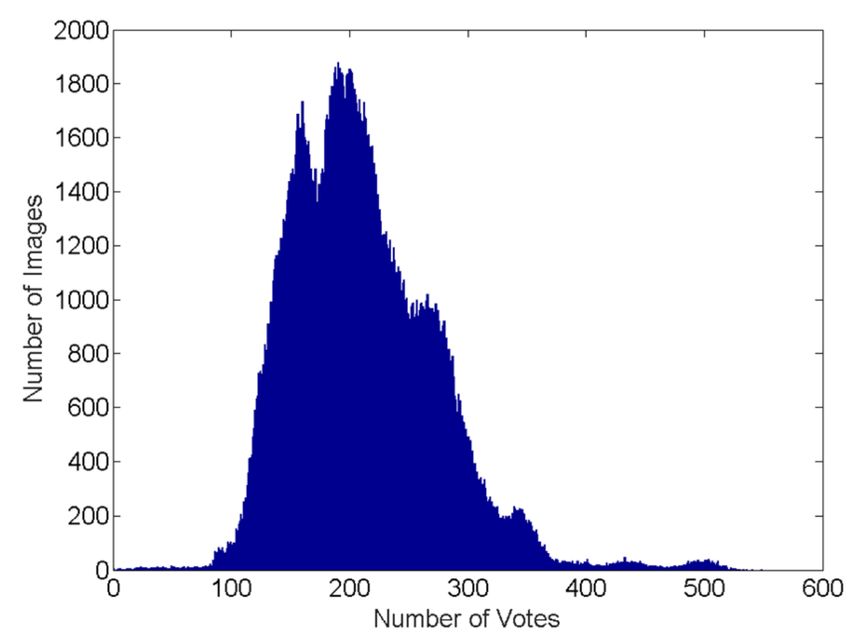
[2] Chaoran Cui, Huidi Fang, Xiang Deng, Xiushan Nie, Hongshuai              [18] Xin Lu, Zhe Lin, Xiaohui Shen, Radomir Mech, and James Z Wang.
     Dai, and Yilong Yin. Distribution-oriented aesthetics assessment for          Deep multi-patch aggregation network for image style, aesthetics,
     image search. In Proceedings of the 40th International ACM SIGIR              and quality estimation. In Proceedings of the IEEE International
     Conference on Research and Development in Information Retrieval,              Conference on Computer Vision, pages 990–998, 2015.
     pages 1013–1016. ACM, 2017.                                              [19] L. McInnes, J. Healy, and J. Melville. UMAP: Uniform Manifold
 [3] Ritendra Datta, Dhiraj Joshi, Jia Li, and James Z Wang. Study-                Approximation and Projection for Dimension Reduction. ArXiv e-
     ing aesthetics in photographic images using a computational ap-               prints, February 2018.
     proach. In European Conference on Computer Vision, pages 288–            [20] Leland McInnes, John Healy, Nathaniel Saul, and Lukas Gross-
     301. Springer, 2006.                                                          berger. Umap: Uniform manifold approximation and projection.
 [4] Yubin Deng, Chen Change Loy, and Xiaoou Tang. Image aesthetic                 The Journal of Open Source Software, 3(29):861, 2018.
     assessment: An experimental survey. IEEE Signal Processing Mag-          [21] Naila Murray and Albert Gordo. A deep architecture for unified
     azine, 34(4):80–106, 2017.                                                    aesthetic prediction. arXiv preprint arXiv:1708.04890, 2017.
 [5] Sagnik Dhar, Vicente Ordonez, and Tamara L Berg. High level de-          [22] Naila Murray, Luca Marchesotti, and Florent Perronnin. AVA: A
     scribable attributes for predicting aesthetics and interestingness. In        large-scale database for aesthetic visual analysis. In 2012 IEEE Con-
     Proceedings of the IEEE International Conference on Computer Vi-              ference on Computer Vision and Pattern Recognition, pages 2408–
     sion, pages 1657–1664. IEEE, 2011.                                            2415. IEEE, 2012.
 [6] Xing Fan, Wei Jiang, Hao Luo, and Mengjuan Fei. Spherereid: Deep         [23] Hamid R Sheikh and Alan C Bovik. Image information and visual
     hypersphere manifold embedding for person re-identification. Jour-            quality. IEEE Transactions on Image Processing, 15(2):430–444,
     nal of Visual Communication and Image Representation, 60:51–58,               2006.
     2019.                                                                    [24] Hossein Talebi and Peyman Milanfar. NIMA: Neural image assess-
 [7] Xin Fu, Jia Yan, and Cien Fan. Image aesthetics assessment using              ment. IEEE Transactions on Image Processing, 27(8):3998–4011,
     composite features from off-the-shelf deep models. In 2018 25th               2018.
     IEEE International Conference on Image Processing (ICIP), pages          [25] Hanghang Tong, Mingjing Li, Hong-Jiang Zhang, Jingrui He, and
     3528–3532. IEEE, 2018.                                                        Changshui Zhang. Classification of digital photos taken by photog-
 [8] Le Hou, Chen-Ping Yu, and Dimitris Samaras. Squared earth                     raphers or home users. In Pacific-Rim Conference on Multimedia,
     mover’s distance-based loss for training deep neural networks. arXiv          pages 198–205. Springer, 2004.
     preprint arXiv:1611.05916, 2016.                                         [26] Zhangyang Wang, Ding Liu, Shiyu Chang, Florin Dolcos, Diane
 [9] Bin Jin, Maria V Ortiz Segovia, and Sabine Süsstrunk. Image aes-             Beck, and Thomas Huang. Image aesthetics assessment using deep
     thetic predictors based on weighted CNNs. In 2016 IEEE Interna-               Chatterjee’s machine. In 2017 International Joint Conference on
     tional Conference on Image Processing (ICIP), pages 2291–2295.                Neural Networks (IJCNN), pages 941–948. IEEE, 2017.
     IEEE, 2016.                                                              [27] Ou Wu, Weiming Hu, and Jun Gao. Learning to predict the per-
[10] Xin Jin, Le Wu, Xiaodong Li, Siyu Chen, Siwei Peng, Jingying Chi,             ceived visual quality of photos. In 2011 International Conference
     Shiming Ge, Chenggen Song, and Geng Zhao. Predicting aesthetic                on Computer Vision, pages 225–232. IEEE, 2011.
     score distribution through cumulative Jensen-Shannon divergence.         [28] Hong-Ming Yang, Xu-Yao Zhang, Fei Yin, and Cheng-Lin Liu. Ro-
     In Thirty-Second AAAI Conference on Artificial Intelligence, 2018.            bust classification with convolutional prototype learning. In Pro-
[11] Xin Jin, Le Wu, Geng Zhao, Xinghui Zhou, Xiaokun Zhang, and                   ceedings of the IEEE Conference on Computer Vision and Pattern
     Xiaodong Li. Idea: A new dataset for image aesthetic scoring. Mul-            Recognition, pages 3474–3482. IEEE, 2018.
     timedia Tools and Applications, pages 1–15, 2018.
[12] Sergey Karayev, Matthew Trentacoste, Helen Han, Aseem Agar-
     wala, Trevor Darrell, Aaron Hertzmann, and Holger Winnemoeller.
     Recognizing image style. arXiv preprint arXiv:1311.3715, 2013.
[13] Shu Kong, Xiaohui Shen, Zhe Lin, Radomir Mech, and Charless
     Fowlkes. Photo aesthetics ranking network with attributes and con-
     tent adaptation. In European Conference on Computer Vision, pages
     662–679. Springer, 2016.
[14] Kwan-Yee Lin and Guanxiang Wang. Self-supervised deep multiple
     choice learning network for blind image quality assessment. In The
     British Machine Vision Conference, page 70, 2018.
[15] Ligang Liu, Renjie Chen, Lior Wolf, and Daniel Cohen-Or. Op-
     timizing photo composition. In Computer Graphics Forum, vol-
     ume 29, pages 469–478. Wiley Online Library, 2010.
[16] Weiyang Liu, Yandong Wen, Zhiding Yu, Ming Li, Bhiksha Raj,
     and Le Song. Sphereface: Deep hypersphere embedding for face
     recognition. In Proceedings of the IEEE Conference on Computer
     Vision and Pattern Recognition, pages 212–220, 2017.
[17] Xin Lu, Zhe Lin, Hailin Jin, Jianchao Yang, and James Z Wang.
     Rapid: Rating pictorial aesthetics using deep learning. In Pro-
     ceedings of the 22nd ACM International Conference on Multimedia,
     pages 457–466. ACM, 2014.

                                                                                              IS&T International Symposium on Electronic Imaging 2020
188-6                                                                                   Imaging and Multimedia Analytics in a Web and Mobile World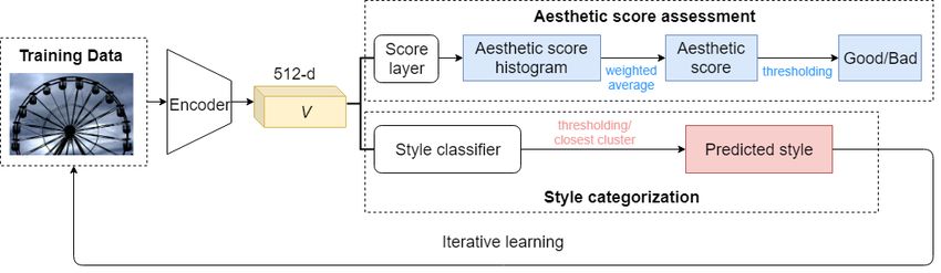
JOIN US AT THE NEXT EI!

 IS&T International Symposium on

 Electronic Imaging
 SCIENCE AND TECHNOLOGY

Imaging across applications . . . Where industry and academia meet!

• SHORT COURSES • EXHIBITS • DEMONSTRATION SESSION • PLENARY TALKS •
• INTERACTIVE PAPER SESSION • SPECIAL EVENTS • TECHNICAL SESSIONS •

                  www.electronicimaging.org
                                                             imaging.org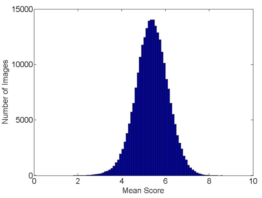
You can also read