Simulating the dynamics and synchrotron emission from relativistic jets II. Evolution of non-thermal electrons
←
→
Page content transcription
If your browser does not render page correctly, please read the page content below
MNRAS 000, ??–?? (2015)                                Preprint 7 May 2021               Compiled using MNRAS LATEX style file v3.0

                                              Simulating the dynamics and synchrotron emission from
                                              relativistic jets II. Evolution of non-thermal electrons
                                              Dipanjan Mukherjee1? , Gianluigi Bodo3 , Paola Rossi3 , Andrea Mignone2 & Bhargav Vaidya                                    4
                                              1 Inter-University Centre for Astronomy and Astrophysics, Post Bag 4, Pune - 411007, India.
                                              2 Dipartimento di Fisica Generale, Universita degli Studi di Torino , Via Pietro Giuria 1, 10125 Torino, Italy
                                              3 INAF/Osservatorio Astrofisico di Torino, Strada Osservatorio 20, I-10025 Pino Torinese, Italy
                                              4 Discipline of Astronomy, Astrophysics and Space Engineering, Indian Institute of Technology Indore,

                                              Khandwa Road, Simrol, 453552, India
arXiv:2105.02836v1 [astro-ph.HE] 6 May 2021

                                              7 May 2021

                                              ABSTRACT
                                              We have simulated the evolution of non-thermal cosmic ray electrons (CREs) in 3D relativistic magneto hydrodynamic
                                              (MHD) jets evolved up to a height of 9 kpc. The CREs have been evolved in space and in energy concurrently with the
                                              relativistic jet fluid, duly accounting for radiative losses and acceleration at shocks. We show that jets stable to MHD
                                              instabilities show expected trends of regular flow of CREs in the jet spine and acceleration at a hotspot followed by
                                              a settling backflow. However, unstable jets create complex shock structures at the jet-head (kink instability), the jet
                                              spine-cocoon interface and the cocoon itself (Kelvin-Helmholtz modes). CREs after exiting jet-head undergo further
                                              shock crossings in such scenarios and are re-accelerated in the cocoon. CREs with different trajectories in turbulent
                                              cocoons have different evolutionary history with different spectral parameters. Thus at the same spatial location,
                                              there is mixing of different CRE populations, resulting in a complex total CRE spectrum when averaged over a given
                                              area. Cocoons of unstable jets can have an excess build up of energetic electrons due to re-acceleration at turbulence
                                              driven shocks and slowed expansion of the decelerated jet. This will add to the non-thermal energy budget of the
                                              cocoon.
                                              Key words: galaxies: jets –(magnetohydrodynamics)MHD – relativistic processes – methods: numerical

                                              1 INTRODUCTION                                                       expanding jet (Longair et al. 1973; Blandford & Königl 1979).
                                                                                                                   The electrons are primarily accelerated at strong shocks in-
                                              Supermassive blackholes at the centres of galaxies can launch
                                                                                                                   side the jet and its cocoon via diffusive shock acceleration (or
                                              powerful relativistic jets that can grow to extragalactic scales.
                                                                                                                   Fermi 1st order processes, Blandford & Ostriker 1978; Drury
                                              These structures have since long been observed in radio fre-
                                                                                                                   1983; Blandford & Eichler 1987). However, recent works (e.g.
                                              quencies, starting from observations of Cygnus A by Jenni-
                                                                                                                   Rieger et al. 2007; Sironi et al. 2021) have also pointed to the
                                              son & Das Gupta (1953). Since early days it had been es-
                                                                                                                   importance of other microphysical processes such as Fermi
                                              tablished that incoherent synchrotron emission by energetic
                                                                                                                   second order and reconnection at shear layers to accelerate
                                              non-thermal electrons in magnetised jets gives rise to the
                                                                                                                   particles to some extent. After an acceleration event, the en-
                                              observed radiation (Shklovskii 1955; Burbidge 1956). Sub-
                                                                                                                   ergetic electrons are expected to suffer cooling due to syn-
                                              sequently, there has been extensive work to understand the
                                                                                                                   chrotron and inverse-Compton losses.
                                              physical nature of these objects (e.g. Blandford & Rees 1974;
                                              Blandford & Königl 1979) and the source of the emission. We
                                              refer the reader to reviews such as Begelman et al. (1984),             Detailed semi-analytic calculations of the evolution of the
                                              Worrall & Birkinshaw (2006) and Blandford et al. (2019) for          energy spectrum of non-thermal electron populations moving
                                              more elaborate discussions on the historical evolution of the        in a fluid flow have been presented in several papers (Karda-
                                              concept of relativistic radio jets and their emission processes.     shev 1962; Jaffe & Perola 1973; Murgia et al. 1999; Hardcas-
                                                 A key factor that strongly affects the emitted radiation is       tle 2013). However, there remain several restrictive assump-
                                              the nature and evolution of the non-thermal electrons inside         tions in such semi-analytic approaches regarding the nature
                                              the jet that gives rise to the synchrotron emission. It had          of the magnetic field distribution experienced by the parti-
                                              again been identified quite early that the electrons must be         cles, the pitch angle of the electron with respect to the mag-
                                              energised inside the jet after ejection from the central nu-         netic field and the location of acceleration. The non-thermal
                                              cleus, to avoid losing energy due to adiabatic losses in the         electrons can experience a wide variety of physical parame-
                                                                                                                   ters of the background environment during their trajectory,
                                                                                                                   which shapes their spectrum. Addressing this requires a fully
                                              ?   dipanjan@iucaa.in                                                numerical approach where the non-thermal electron popula-

                                              © 2015 The Authors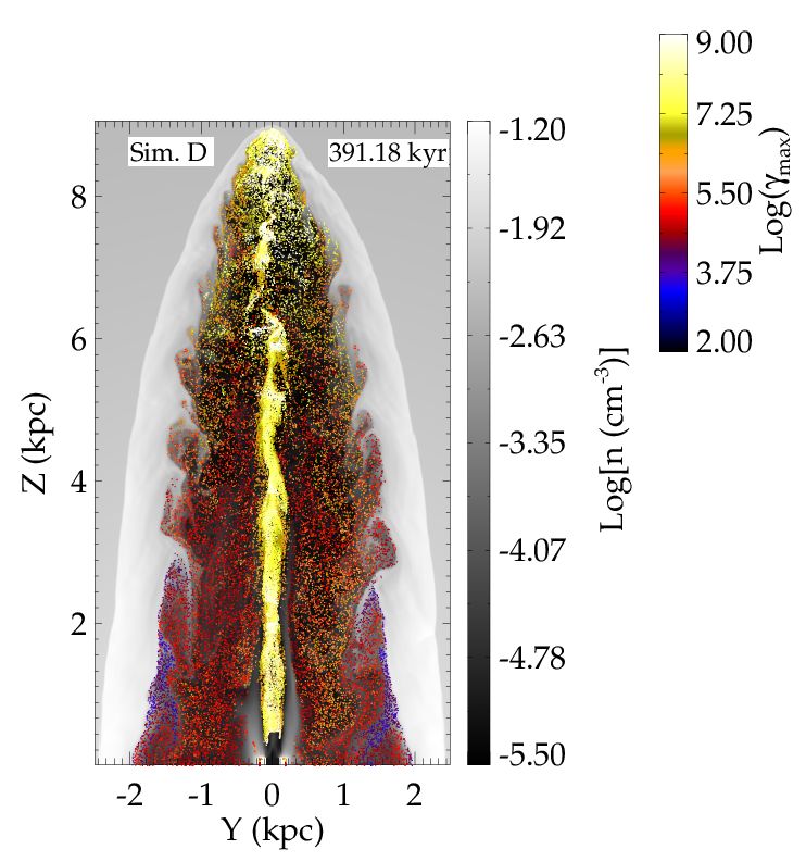
2     Mukherjee et al.
tion are allowed to sample the local properties of the fluid,      advected spatially following the fluid motions. Their energy
as opposed to averaged quantities.                                 is found by evolving their phase space distribution function,
   In some recent works, numerical simulations have been pre-      duly accounting for energy losses due to radiative processes
sented that self-consistently evolve spectra of non-thermal        such as synchrotron emission and inverse-Compton interac-
electrons concurrently with the fluid (viz. Jones et al. 1999;     tion with CMB photons. Appendix A1 briefly summarises the
Micono et al. 1999; Mimica et al. 2009; Fromm et al. 2016;         method of phase space evolution of a CRE.
Vaidya et al. 2018; Winner et al. 2019; Huber et al. 2021).
The standard approach involves solving the phase space evo-
lution of the non-thermal electrons while accounting for ra-       2.1 Diffusive shock acceleration
diative losses and acceleration due to microphysical processes
                                                                   Electrons crossing shocks can be accelerated to higher en-
such as diffusive shock acceleration. However, such meth-
                                                                   ergies via diffusive shock acceleration (hereafter DSA, see
ods have been applied to study astrophysical jets in radio
                                                                   Blandford & Ostriker 1978; Drury 1983, for a review). The
galaxies by only a handful of papers, and with restrictive as-
                                                                   DSA theory predicts that particles exiting a shock can have a
sumptions. For example, Jones et al. (1999); Micono et al.
                                                                   power-law spectrum whose index depends on the shock com-
(1999); Tregillis et al. (2001) have simulated the evolution
                                                                   pression ratio defined in Eq. (A7). The maximum energy of
of non-thermal electrons in large scale jets but in a non-
                                                                   the resultant spectrum is found by equating the time scale of
relativistic framework. Other works have evolved the non-
                                                                   Synchrotron driven radiative losses to the acceleration time
thermal electrons embedded in relativistic fluid (e.g. Mimica
                                                                   scale (as given in Eq. (A8)). For relativistic shocks, power-law
et al. 2009; Fromm et al. 2016), but for small parsec scale
                                                                   index of the spectrum is calculated differently for parallel1
quasi-steady state jets, without exploring the detailed evolu-
                                                                   and perpendicular shocks, as in Eq. (A10) and Eq. (A11).
tion up to larger distances (kpc), which is relevant for jets in
                                                                   Further details of the above steps are summarised in Ap-
radio galaxies.
                                                                   pendix A. In the next sections we describe an empirical
   In this series of papers, we will study the properties of
                                                                   approach to obtain the downstream spectrum of a shocked
the non-thermal electrons, evolved concurrently with the rel-
                                                                   CRE.
ativistic jet fluid, while duly accounting for the radiative en-
ergy losses and acceleration at shocks (Vaidya et al. 2018).
The current paper, second in the series, presents the be-          2.1.1 Previous approaches of evaluating shocked spectra
haviour and evolution of the non-thermal electrons along with
the bulk relativistic jet flow for different simulations with a    In several previous similar works (e.g. Mimica et al. 2009;
wide range of jet parameters. The results on the dynamics of       Böttcher & Dermer 2010; Fromm et al. 2016; Vaidya et al.
these simulated jets have been presented earlier in (Mukher-       2018), the spectrum of shock accelerated particles were re-
jee et al. 2020). In subsequent papers we shall discuss the        set to a power-law with an index predicted by the theory of
impact on observations (synchrotron and inverse-Compton)           DSA. This would result in the particles losing the history of
expected from such simulated jets.                                 their spectra before the entering the shock. The normalisa-
   The plan of the paper is as follows. In Sec. 2 we summarise     tion of the spectra and the lower-limit (Emin ) were set by
the implementation of the method to solve for the evolution        enforcing the particles to have a fractional energy and num-
of non-thermal electrons presented in Vaidya et al. (2018)         ber density of the fluid. However, this has the following two
and new changes introduced in this paper in the modelling of       disadvantages.
diffusive shock acceleration. In Sec. 3 we discuss the numeri-
                                                                      • In complex simulations with multiple shock features, a
cal details of injection of non-thermal electrons. In Sec. 4 we
                                                                   single computational cell may host more than one particle,
briefly summarise the results of the dynamics of the simu-
                                                                   and only a fraction of them may have crossed a shock. Some
lated jets, which have been presented in detail in Mukherjee
                                                                   CRE macro-particles may have been advected to the cell
et al. (2020). In Sec. 5 we discuss the results of the spatial
                                                                   without crossing a shock, by different flow stream lines. Ad-
and spectral evolution of the non-thermal electrons and how
                                                                   ditionally there can be multiple particles that exit the same
they vary for different simulations with different jet parame-
                                                                   shock feature at the same time, thus requiring a simultane-
ters. In Sec. 6 we summarise our results and discuss on their
                                                                   ous spectral update. Hence, in a departure from Vaidya et al.
implications.
                                                                   (2018), where each particle was assigned an energy of fE ×ρ,
                                                                   we distribute to the newly shocked particles in the cell only
                                                                   the energy remaining after subtracting from fE × ρ the ex-
2 EVOLUTION OF THE COSMIC RAY                                      isting cosmic ray energy density .
  ELECTRONS                                                           • Secondly, resetting the spectrum to a new power-law re-
                                                                   sults in total loss of the spectral history of previous shock en-
In Vaidya et al. (2018, hereafter BV18) a detailed analytical      counters. Such multiple shock crossings can leave an imprint
and numerical framework was developed to evolve a distribu-        on the final spectra due to different acceleration time scales
tion of non-thermal particles both spatially and in momen-         and power-law indices generated at different shocks (e.g. Mel-
tum space. This was introduced as the Lagrangian Parti-            rose & Pope 1993; Micono et al. 1999; Gieseler & Jones 2000;
cle module in the PLUTO code (Mignone et al. 2007). This           Meli & Biermann 2013; Neergaard Parker & Zank 2014). This
module has been applied in the current work to study the evo-
lution of non-thermal electrons in relativistic jets. The non-
thermal relativistic electrons at a region in space are modelled   1 A parallel shock has its normal close to the down-stream mag-
as ensembles of macro-particles which we refer to as a cosmic      netic field. The shock normal and downstream magnetic field are
ray electron macro-particle or CRE in short. The CRE are           at large angles for perpendicular shocks.

MNRAS 000, ??–?? (2015)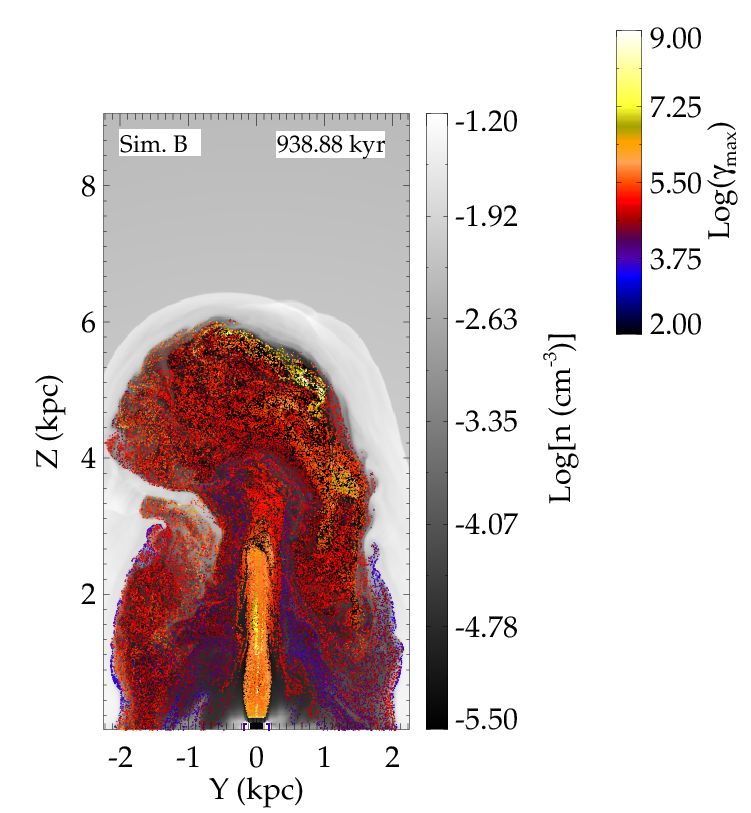
Evolution of non-thermal electrons                    3
is especially problematic in a scenario where a particle hav-      the total energy density of all CREs in the cell should be
ing crossed a strong shock (higher shock compression ratio r),     a fraction fE of the fluid internal energy density2 . We thus
subsequently passes through a weaker shock with a steeper          first compute the total available energy in a computational
power-law index as per DSA theory. Replacing the earlier           volume that may be distributed amongst the newly shocked
shallower spectrum with a new steeper power-law, will result       particles:
in an artificial loss of energy of the CRE macro-particle.                                               X
                                                                                     ∆E = fE × (ρ) −       εi ,             (2)
  To overcome the above limitations we introduce a empiri-                                                   i
cal approach to update the spectrum of a shocked CRE, as           Here (ρ) is the fluid internal energy density, given by
outlined in the next section.
                                                                       ρ = p/(Γ − 1)   (Ideal EOS)                               (3)
                                                                                        2
                                                                                           p
2.1.2 A empirical convolution based approach for updating              ρ = (3/2)p − ρc + (9/4)p2 + ρ2 c4            (T-M EOS),   (4)
      CRE spectra                                                  where Eq. (4) is valid for the Taub-Mathews (T-M) equation
A particle enters a shock with an up-stream (pre-shock) spec-      of state (Taub 1948; Mignone & McKinney 2007).
trum Nup (E). On exiting the shock, the distribution is up-           The energy
                                                                            R     density of a single CRE macro-particle is given
dated to a down-stream (post-shock) spectrum Ndn (E) as:           by εi = EN (E)dE. Freshly shocked particles that are to be
                                                                   updated are excluded from the summation in the second term
                                                     dE 0
                      Z E
                                                                   of Eq. (2). For ∆E > 0, the difference in energy is equally
        Ndn (E) = C         Nup (E 0 )GDSA (E, E 0 ) 0
                       Emin                           E            distributed to all shocked particles in the computational cell,
                                        −q+2                     which sets the value of the normalisation C in Eq. (1). For
                                                    dE 0
                      Z E
                                        E
                  =C        Nup (E 0 )    0
                                                          (1)      ∆E 6 0, no new particles are updated inside the given cell,
                       Emin             E           E0
                                                                   as the CRE energy density of existing particles have already
In Eq. (1) above, Nup (E) is convolved with a function             reached the threshold of fE × (ρ).
GDSA (E, E 0 ) = (E/E 0 )−q+2 , for E ∈ (Emin , Emax ). The min-      • Step2: Subsequently, we compute
imum energy Emin is kept fixed to the minimum energy of                                                     X T
                                                                                  ∆N = fN × ρ/(µma ) −          Ni ,          (5)
the up-stream spectrum. The maximum energy Emax is com-
                                                                                                                 i
puted from Eq. (A8) and Eq. (A9) and the spectral index q
from Eq. (A10) and Eq. (A11).                                      which is the difference between the fluid number density mul-
   For non-relativistic shocks, Eq. (1) with C = q and q =         tiplied by a mass fraction fN and the total number den-
3r/(r − 1), is an exact representation of the down-stream          sity of all CREs in the cell, including that of shocked par-
spectrum (Blandford & Ostriker 1978; Drury 1983), obtained         ticles calculated in step 1 above. Here ma is the atomic mass
by solving for the phase space distribution function of the        unit and µ = 0.6 is the mean molecular weight for ionised
particles across the shock front. In the present work we ex-       gas. TheR number density of a CRE particle is obtained from
tend this as a phenomenological approach to update the up-         NiT = N (E)dE. For ∆N < 0, the normalisation C is re-
stream spectrum of relativistic shocks. The methodology of         duced to ensure that the total cosmic ray electron number
Eq. (1) is similar to the implementation of re-accelerated         density in a computational cell is Ne = fN × ρ/(µma ).
particles in Micono et al. (1999) and Winner et al. (2019).           To summarise, the normalisation is first set to preserve the
Approximate analytical solutions of the particle distribution      energy densities of the particles to be a fraction of (fE ) the
at a relativistic shock without an incident source, predicts a     fluid energy density. Additionally, if the chosen normalisation
power-law spectrum for the downstream particles (Takamoto          results in the CRE number density becoming higher than
& Kirk 2015). Convolving the up-stream spectrum with such          a fraction (fN ) of the fluid number density, the previously
a power-law distribution is thus an empirical approach that        obtained normalisation is lowered to ensure an exact match.
accounts for the spectrum of the incident distribution, as a       In that case, the total CRE energy density will be lower than
CRE exits a shock. Appendix A2.2 has further details regard-       the threshold of fE × ρ, due to a lower value of the new
ing the choice of the power-law index predicted from the DSA       normalisation. Thus the above two-step procedure ensures
theory.                                                            that the CREs have energies and number densities that are
   The above scheme is also similar in nature to the imple-        within the prescribed fractions fE and fN for energy and
mentation of shock acceleration in Jones et al. (1999) and         mass respectively. For this work we have assumed fE = fN =
Tregillis et al. (2001), where the spectrum in an energy bin       0.1.
has been updated only if the index of the local piece-wise            We must note here that chosen fractions are somewhat
power-law is lower than that predicted by DSA. This duly           arbitrary, although not far from the indications obtained
avoids artificial steepening of spectra when energised parti-      from PIC simulations (see e.g. Sironi et al. 2013; Caprioli
cles with flatter spectrum crosses a weak shock, which is also     & Spitkovsky 2014; Guo et al. 2014; Marcowith et al. 2016,
naturally taken care of by the convolution process used here,      2020). In addition, though small, they are not negligible. In
as also elaborated later in this section.                          reality, CREs accelerated at shocks will subtract the corre-
   The normalisation constant C is set in two steps, which         sponding fractional gain in energy from the fluid internal
ensure that the maximum local energy and number density
of the CREs are less than or equal to a specified fraction of
                                                                   2 It is to be noted that as a particle exits a shock into the down-
the fluid.
                                                                   stream region, there may exist other particles inside the compu-
  • Step 1: At computational cells where CREs are to be            tational cell which may have been advected there without passing
updated on exiting the shock, we enforce the criterion that        through a shock, or are remnants of a previous shock-exit.

                                                                                                         MNRAS 000, ??–?? (2015)
4        Mukherjee et al.

                                   Convolution of particle spectrum                          2 CRE particles       Z axis
                            100
                                                              Downstream
                                                                                            injected in 1 cell
                          10−5                                Upstream                                                               V
                                                              DSA (q: 7.0)
                          10−10

                          10−15
     Normalised spectra

                          10−20

                          10−25
                                                                                       Rj

                          10−300
                           10                                                                                      (0,0,0)
                                                                                                                                         X axis
                          10−5
                                                                                                          Rj
                      10−10

                      10−15

                      10−20                                   Downstream                                           Θ
                                                              Upstream
                            −25
                      10                                      DSA (q: 3.0)

                      10−30
                          102      103    104    105    106      107         108               V                                    V
                                                  γ

Figure 1. A demonstration of the empirical scheme involving con-                   Figure 2. A representation of the injection zone of the jet in the
volution of the particle spectrum with the DSA predicted power-                    simulation domain (similar to Fig. 2 of Mukherjee et al. 2020),
law function (in dashed). The up-stream spectrum (in black) of the                 which also shows the injection of the cosmic ray electron (CRE)
particle before the shock update is a power-law with an exponen-                   macro-particles. Two CREs, represented in red, are injected at ev-
tial cut-off given by Eq. (6). The resultant down-stream spectrum                  ery time step in a computational cell (denoted by the black boxes)
(in red) is obtained from their convolution.                                       just above the jet inlet, along the Z axis. The area of injection
                                                                                   spans up to the extent of the jet radius in the X − Y plane. For
                                                                                   one sided jets, CREs are injected only along the upper surface of
energy, which is not considered here. Feedback from radia-
                                                                                   the injection zone, as demarcated here. For twin jets (simulation
tive losses due to non-thermal particles can change the shock                      E), CREs are injected along both upper and lower surfaces.
structure, as demonstrated in Bromberg & Levinson (2009)
and Bodo & Tavecchio (2018). Such effects are not considered
in this work as the CRE particles are considered to be pas-
sively evolving with the fluid. However, given that the CRE                        the higher energies with an initial exponential decay, gets
energy and mass fractions are restricted to a maximum of                           populated with a power-law spectrum of N ∝ γe−7 . Similarly,
10%, the effects are not expected to be substantial, and the                       for a convolution with a power-law function of N ∝ γe−3 , the
qualitative trends are not expected to be affected. Under-                         resultant spectrum yields a power-law of N ∝ γe−3 for the
standing the quantitative impact of energy losses and cosmic                       whole range.
ray pressure requires detailed modelling of the interaction of
the CRE with the fluid and will be deferred to a future work.
   The above procedure to update the spectrum of a shocked
CRE is better at accounting for situations where a CRE has
traversed multiple shocks of different strengths. The convo-
                                                                                   3 NUMERICAL IMPLEMENTATION OF CRE
lution procedure introduced here (as also in Micono et al.
                                                                                     INJECTION
1999; Winner et al. 2019) will redistribute lower energy elec-
trons to higher energy bins as per the functional form of the                      We have performed a series of simulations of relativistic jets
spectrum predicted by DSA. This may be interpreted as the                          expanding into an ambient medium in Mukherjee et al. (2020,
lower energy electrons being accelerated to higher energies.                       hereafter Paper I). In this section we summarise the details of
Thus in the previously described situation of a particle pass-                     how CRE macro-particles are introduced into the simulation
ing first through a stronger shock followed by a weaker one,                       domain. We refer the reader to Sec. 2 of Paper I for details
the resultant spectrum would be a broken power-law.                                regarding the magneto-hydrodynamics of the simulation and
   The top panel of Fig. 1 demonstrates two possible scenarios                     related information regarding the simulation set up.
of shock crossing by a CRE. Here the up-stream spectrum is                           The CRE are injected in the simulation in computational
given by a power-law with an exponential cut-off:                                  zones just above the inlet of the jet along the Z axis, as

                                     γe
                                                                                  shown in Fig. 2. Two CRE particles were injected at each
                    N ∝ γe−α exp −        ,                (6)                     cell, at each time step, to achieve greater filling of the cocoon
                                     γc
                                                                                   volume. The injected particles are immediately advected by
with α = 5 and γc = 104 representing the slope at lower en-                        the jet flow upwards along the jet axis. Over the course of the
ergies and cut-off energy respectively. The resultant convolu-                     simulations, typically several million particles are injected, as
tion with a spectrum of N ∝ γe−7 , gives a broken power-law,                       shown by the last column in Table 1.
as shown in the upper panel of Fig. 1. The lower energies                            At injection the CRE macro-particles are initialised with
below the break remain a power-law with N ∝ γe−5 , whereas                         a steep power-law spectrum (α1 = 9) and limiting Lorentz

MNRAS 000, ??–?? (2015)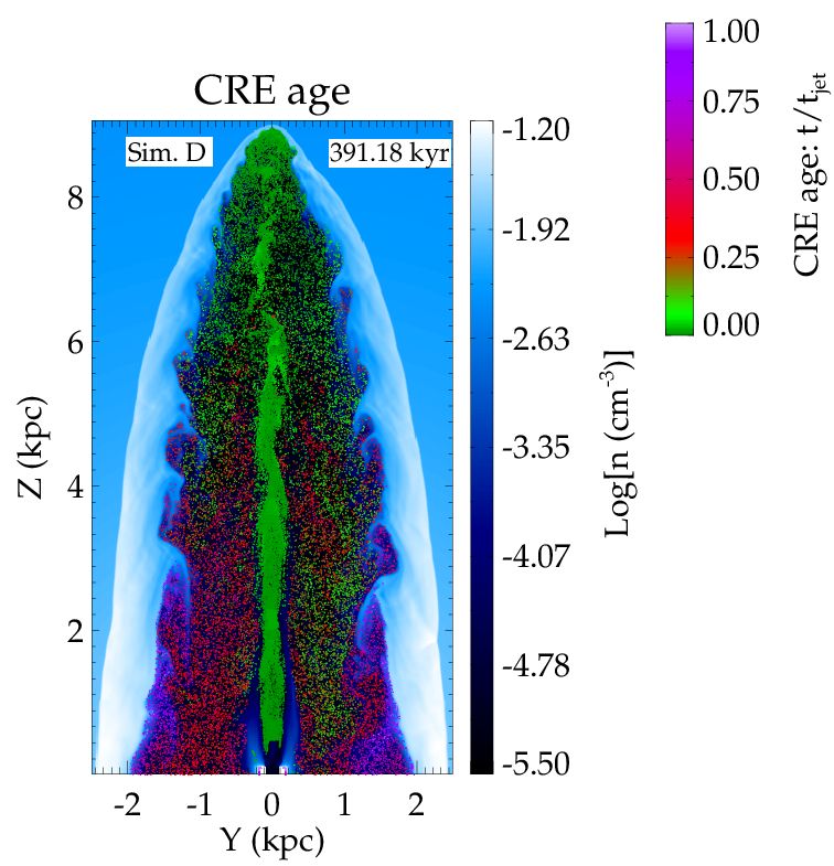
Evolution of non-thermal electrons                 5

Table 1. List of simulations and parameters                                    the same nomenclature of the simulations as done in Pa-
                                                                               per I, for consistency. The simulations probe a wide range
       Sim.    γj       σB          Pj           No. Particlesa                of jet parameters, namely: jet power (Pj ), jet magnetisation
       label                   (1045 ergs−1 )       (×106 )                    (σj ) and the bulk Lorentz factor (γj ). Broadly we can divide
                                                                               the results into three groups: simulation B with a low power
       Bb      3     0.1            0.2                   16.4                 jet (Pj ∼ 1044 erg s−1 ), simulations D, E, F with moderate
       D       5     0.01           1.1                   6.5
                                                                               power jets (Pj ∼ 1045 erg s−1 ) and simulations G, H, J with
       E        5    0.05           1.2                   18.0
       F       5     0.1            1.2                   3.2
                                                                               high power jets (Pj ∼ 1046 erg s−1 ). In most simulations the
       G        6     0.2           8.3                   14.9                 jets were followed up to 9 kpc, except for simulation J where
       H       10    0.2           16.4                    9.8                 the domain is larger.
       J       10     0.1          15.1                   55.3                    In Paper I, we have discussed the dynamics of the jets. One
                                                                               of the primary results of the paper, which is also strongly rel-
 a The total number of particles injected during the course of the
                                                                               evant for the discussion in the current work, is the onset of
simulation.                                                                    different MHD instabilities for different ranges of jet parame-
 b The density contrast defined as the ratio of the jet density to
                                                                               ters. We summarise briefly below the main findings of Paper
ambient gas is 4 × 10⁻⁵ . For all other cases, the value is η = 10−4
                                                                               I which are relevant to the present work.
Parameters:
 γb :  Jet Lorentz factor.                                                        (i) Kink unstable (simulation B): Simulation B with a
 σB : Jet magnetisation, the ratio of jet Poynting flux                        low power jet (Pj ∼ 1044 erg s−1 ) and strong magnetisation
       to enthalpy flux. See eq. (7) of Paper I.                               (σB ∼ 0.1) is unstable to kink mode instabilities. The kink
 Pj :  Jet power. See eq. (9) of Paper I.                                      instabilities cause the jet axis and head to bend strongly,
                                                                               which creates complex shock structures at the jet head (see
factors: (γmin , γmax ) ≡ (102 , 106 ) as                                      Fig. 4 in Paper I).
                                                                                (ii) KH unstable (simulation D): Jets with lower mag-
                                   1 − α1
            N (E) = nm         1−α1       1−α1   E −α1                   (7)   netisation, such as simulation D with Pj ∼ 1045 erg s−1 and
                             Emax     − Emin                                   σB = 0.01, suffer from Kelvin-Helmholtz (hereafter KH) in-
                      Z Emax
                                                                               stabilities. This decelerates the jet and creates turbulence
             where            N (E)dE = nm                               (8)
                        Emin                                                   inside the jet and cocoon, with a disrupted jet-spine due to
                                                                               vortical fluid motions resulting from the KH modes.
Here nm is the CRE number density, whose value is set as
                                                                                  (iii) Stable jets (simulations F,H): Moderate to high
follows. With npi CRE particles injected in a computational
                                                                               power jets (Pj ∼ 1045 − 1046 erg s−1 ) with stronger magneti-
cell with volume ∆V , the total energy of the injected CREs
                                                                               sation (σB ∼ 0.1) remain stable to both kink and KH modes
is
              Z Emax                                                           up to the run time of the simulations explored in these works,
  Ei = npi ∆V        EN (E)dE                            (9)                   such as simulations F and H. This is due to reduced growth
                 Emin                                                          rates of KH modes due to stronger magnetic field and also

                             α1 − 1

                                                           Γ
                                                                              reduced growth of both kink and KH modes due to higher
    ' npi nm me c2 ∆V                     γmin = fE                  pj ∆V,    bulk Lorentz factors.
                             α1 − 2                       Γ−1
                                                                        (10)      (iv) Turbulent cocoon (simulation G): Higher pres-
                                                                               sure of the jet results in more internal structure. The higher
where γmax  γmin has been assumed. The last equality in                       sound speed facilitates the growth of small scale perturba-
Eq. (10) arises from assuming that the CRE energy density                      tions (Rosen et al. 1999), which can develop internal shocks
in the volume ∆V accounts for a fraction fE of the fluid                       and turbulence. Simulation G (Pj ∼ 1046 erg s−1 ) with an
enthalpy in rest frame. The jet pressure is given by pj . Sim-                 injected jet pressure five times that of simulation H, shows
plifying Eq. (10), we get the CRE number density as                            such internal instabilities and turbulence.

                       Γ      (α1 − 2)      pj
          nm = fE                                  .      (11)                   In the rest of the paper, a major theme would be to explore
                     Γ − 1 (α1 − 1) npi γmin me c2                             the effect of the above different MHD instabilities on the
  However, one must note that the starting configuration of                    evolution of the CREs.
the CRE spectrum defined in Eq. (7) and Eq. (11) is renewed
when they encounter the first shock, which occurs fairly close
to the injection surface, from the recollimation shocks within
the jets. Thus the resultant spectra of the particles inside                   5 RESULTS
the main jet flow after some distance away from the injection
surface are insensitive to the initial values.                                 According to the standard evolutionary picture, CREs are
                                                                               considered to be carried by the jet up to the termination
                                                                               shock at the jet-head, and eventually follow the back-flow in
                                                                               the cocoon to lower heights, as shown in Fig. 3. The particles
4 REVIEW OF RESULTS FROM PAPER I
                                                                               are expected to be accelerated to high energies with a shallow
In Mukherjee et al. (2020, Paper I) we have presented the                      power-law spectrum at the jet-head and subsequently cool
results of the simulations of relativistic jets, focusing on the               down in the backflow inside the cocoon due to radiative losses
evolution of the dynamics and fluid parameters in the jet                      from synchrotron and inverse-Compton interaction with the
and its cocoon. Table 1 lists the simulations where the non-                   CMB radiation (Jaffe & Perola 1973; Murgia et al. 1999; Har-
thermal CREs were evolved along with the fluid. We keep                        wood et al. 2013, 2015; Hardcastle 2013). However, the above

                                                                                                                   MNRAS 000, ??–?? (2015)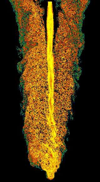
6     Mukherjee et al.

                                 Forward shock
                                                                                                    Sim. H
         Contact discontinuity

                Cocoon
                                                                                  9                                  20
                                         CRE trajectory                           8                P3
                                                                                  7
                  Jet-spine
                                                          Hotspot
                                                                                                                     15

                                                                                                                         Number of shocks
                  Recollimation shocks
                                                                                  6                     P4
                                                                                  5

                                                                            z [kpc]
                                                                                                                     10
                                                                                  4                   P2
                                                                                  3
Figure 3. A schematic showing the structure of the jet spine, the                                                    5
cocoon surrounding it, the contact discontinuity and the forward                  2        P1
shock. The non-thermal electrons (called here as cosmic ray elec-
trons or CREs) are expected to travel first through the jet spine                 1                                  1
up to the hotspot and flow back down into the cocoon. The CREs
are first accelerated at the sites of recollimation shocks (Norman
et al. 1982; Komissarov & Falle 1998) inside the jet before they

                                                                                      1
reach the strong shock at the hotspot.

                                                                                       0                   1
                                                                                  y [k
picture is simplistic, especially for complex flow patterns aris-
                                                                                           1 1 0
                                                                                      pc]
                                                                                                x [kpc]
ing out of MHD instabilities in the jet and the cocoon. In the
following sub-sections, we describe the behaviour of the par-
ticles as they evolve with the jet and highlight the differences
from the above standard paradigm.                                    Figure 4. Trajectories of 4 representative particles (named P1,
                                                                     P2, P3 and P4) that undergo multiple shocks in simulation H.
                                                                     The color of the particles show the number of shocks crossed at a
5.1 Evolution of CREs in the jet and cocoon                          given point of the track.

5.1.1 CREs in stable powerful jets
                                                                     evolutionary picture proposed in earlier works (e.g. Jaffe &
In this section we describe the coevolution of the CREs with
                                                                     Perola 1973; Komissarov & Falle 1998; Turner & Shabala
the jet for case H, a prototypical stable jet with Pjet =
                                                                     2015), as also summarised in the schematic in Fig. 3.
1046 erg s−1 . The CREs injected at each time step (as out-
lined in Sec. 3) are advected along with the jet flow till they
reach the jet head. There, the CREs interact with the termi-
                                                                     5.1.2 Impact of MHD instabilities
nation shock and turn back into the cocoon pushed by the
jet’s back-flow. This is well demonstrated by the trajectories          • Simulation B, kink unstable: Simulation B with a lower
of four representative CREs in Fig. 4. The chosen particles          jet power (Pj ∼ 1044 erg s−1 ) shows a uniform distribution
from four different heights at the end of the simulation have        of maximum Lorentz factor, as shown in the upper panel
the largest number of shock crossings at the given heights.          of Fig. 6. This is in sharp contrast to that of simulation H
   The CREs are first accelerated inside the jet spine itself,       (Fig. 5), where the high values of γmax are concentrated at
at the several recollimation shocks, before they reach the jet       the locations of the strong shocks in the jet axis and the
head. This causes the particles to attain a large value of max-      jet-head. The kink instabilities result in the bending of the
imum Lorentz factor γmax inside the jet axis. This can be seen       jet head, ultimately leading to the formation of an extended
in the top panel of Fig. 5, where we present the CREs with           termination shock spreading horizontally from the main axis
color scaled to the value of log(γmax ), over-plotted on the den-    of the jet (see top panel in Fig. 7). CREs traversing such
sity profile in the Y − Z plane. The bottom panels of Fig. 5         shock will undergo complex shock crossings. For example,
show the particles coloured by time lapsed since last shock          the paths of P1 and P3 are sharply twisted as they encounter
encounter. The CREs within the jet axis are also seen to be          the complex shocks at the jet head. They undergo several
young in age as they have been relatively recently shocked at        shock crossings after they exit the jet axis, evidenced from
the sites of recollimation.                                          the rapid change in the color in the lower panel of Fig. 6.
   Once the particles reach the jet-head, they cross the strong         The instabilities also strongly decelerate the jet. This re-
shock at the Mach-disk and follow the backflow of the jet            sults in constant injection of energetic CREs into the slowly
into the cocoon. The cocoon has older particles, represented         inflating cocoon. CREs exiting the jet at different heights, lie
in magenta and red in Fig. 5. The CREs in the cocoon also            close together near the base (e.g. particles P2 and P3). Such
have lower maximum energies as they lose energy steadily             CREs are further re-accelerated at other shock surfaces due
due to radiative losses. Thus the CREs in this simulation of         to internal turbulence and the complex back-flow. For exam-
a jet stable to MHD instabilities conform well to the standard       ple, particle P3 (right panel of Fig. 6) gets further shocked

MNRAS 000, ??–?? (2015)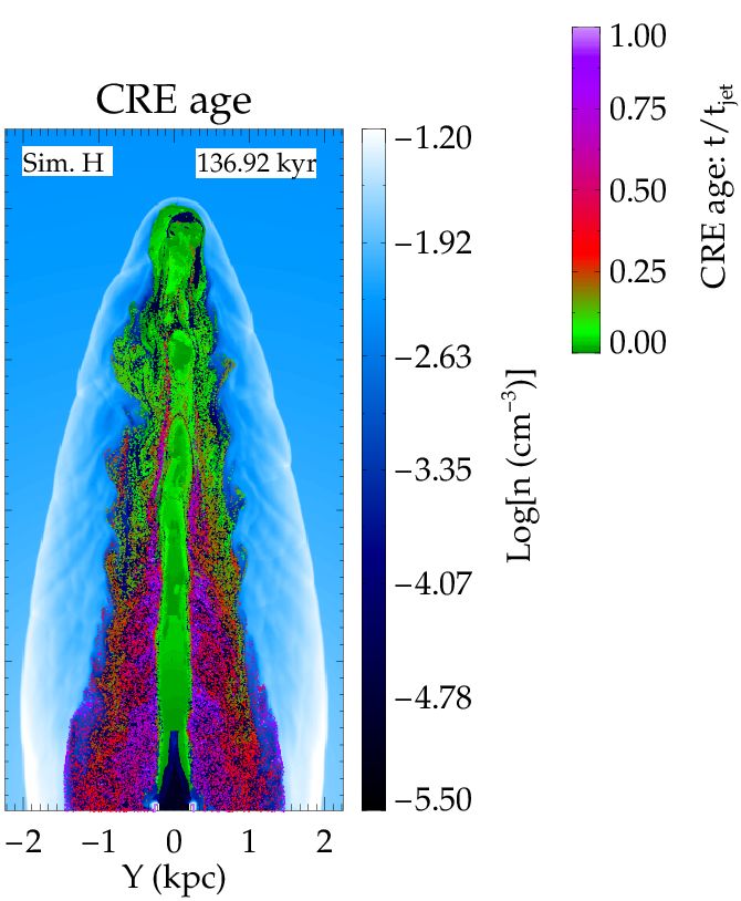
Evolution of non-thermal electrons 7
necting the locations at different times, is seen to perform a
loop at Z ∼ 3 kpc, before reaching to a maximum height of
Z ∼ 5 kpc and subsequently streaming down. CRE P2 simi-
larly show a complex trajectory (in blue) with a vertical rise
up to Z ∼ 6 kpc, a backward motion thereafter, and again
a rise up to Z ∼ 8 kpc. These vortical motions of the CREs
result from the onset of Kelvin-Helmholtz instabilities at the
jet-cocoon interface.
What is noteworthy here, is that the cause for the multi-
ple shock crossings in simulation D is fundamentally different
than that in simulation B. In simulations B and H, the CREs
are shocked multiple times due to the geometry of the shock
structure at the jet head, beyond which they stream down
along the back flow, with some exceptions. The CREs in sim-
ulation D encounter multiple weaker shocks within the body
of the cocoon itself as they stream down along the backflow
and also at the outer layer of the jet-spine where KH driven
vortices arise, leading to turbulence and shocks.
Thus a more extended region of the cocoon is filled with
freshly shocked younger electrons, as shown in middle panel
of Fig. 8. Similarly from the right panel of Fig. 8 it can be seen
that the CREs inside the cocoon are shocked to higher ener-
gies, in sharp contrast to that in simulation H (Fig. 5). This is
because the magnetic field in simulation D is almost an order
of magnitude lower than that in H, resulting in longer syn-
chrotron cooling time scales (see Eq. (A8)), allowing efficient
acceleration.
5.2 History of the magnetic field, γmax and shock
compression ratio traced by CREs
MHD instabilities can create turbulence in the jet cocoon,
Figure 5. Top panels: Density slices in the X − Z plane for resulting in inhomogeneous distribution of magnetic and ve-
simulation H at two different times. Over-plotted on the density locity fields. Thus, depending on their trajectories in the
maps are particles with colors representing the log(γmax ), where jet-cocoon, different CRE particles may experience varied
γmax is the highest Lorentz factor of the CRE spectrum Bottom evolutionary history. In Fig. 9 we present the variation of
panels: Density slices in the X − Z plane with the CRE positions the magnetic field, the maximum Lorentz factor of the CRE
over-plotted. The color of the CRE represent the time since last spectrum (γmax ) and the shock compression ratio of the last
shock, normalised to the time of the simulation. Freshly shocked shock crossed, for some of the representative particles already
particles (greenish hue) are near the jet head, with older particles
shown in Fig. 4, Fig. 6 and Fig. 8. The variation of these
(purple/pink) at the base.
quantities along the CRE trajectory will leave their imprint
on the CRE energy spectrum.
after exiting the jet axis due to internal shocks inside the co- • Simulation B: The left column of Fig. 9 shows the evo-
coon. Thus there is mixing of particles with different shock lution of physical properties for particles P2 and P3, whose
histories, and the cocoon of a decelerating slowly inflating trajectories have been presented in Fig. 6. We firstly notice
jet is more evenly distributed with shocked highly energetic that although the two particles have similar trajectories, they
particles. encounter very different magnetic fields. Particle P3 shows a
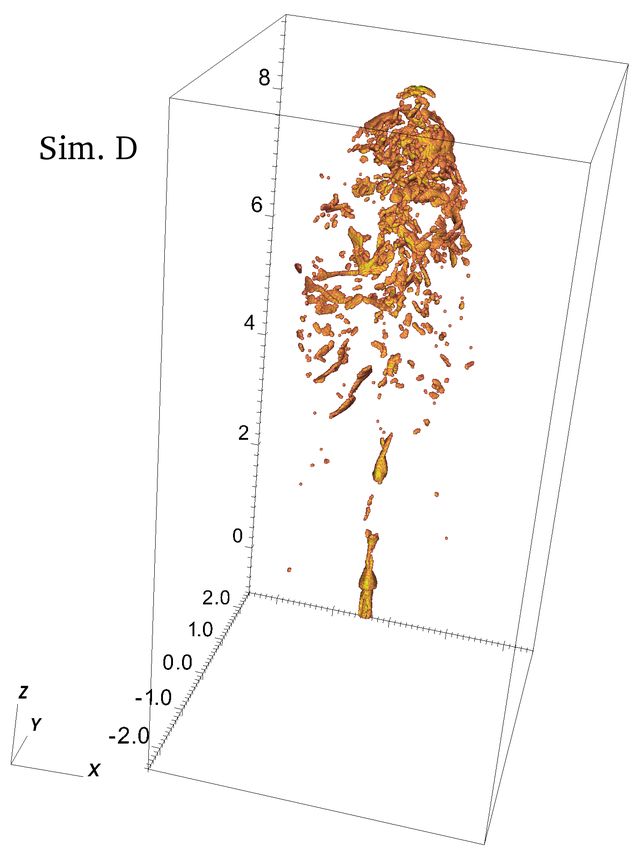
• Simulation D, KH unstable: Simulation D with Kelvin- sharp increase to about ∼ 0.2 mG, followed by a decline,
Helmholtz instabilities has multiple internal shocks inside the and similar subsequent spikes, although of lower magnitudes.
cocoon, as shown in the 3D volume rendering of the shocks The rapid increase in the magnetic fields correlate well with
in Fig. 7. The shock surfaces are identified by computing the changes in the shock-compression ratio, indicating that such
maximum pressure difference at each grid point, as defined sudden increase results from the CRE traversing different
in Eq. (A5). Similar complex web of shock structures have shocks during its trajectory. The γmax also shows similar cor-
also been reported in Tregillis et al. (2001). CREs streaming related increase to high values, followed by an exponential
down the backflow will have to cross these shocks and be re- decline after the last shock. It is interesting to note that since
accelerated in the process. CREs shocked multiple times are its injection after ∼ 650 kyr of the simulation run time, CRE
trapped within this shock layers. P3 experiences multiple shocks for ∼ 200 kyr, before enter-
The above situation is clear by inspecting the complex tra- ing a steady quiescent backflow without shocks. This is due
jectories of the CREs in the left panel of Fig. 8, where the to the complex shock structure created by the kink unstable
paths of two representative CREs have been plotted. CRE bending jet-head.
P1 with the particle trajectory presented in red lines con- CRE P2 however, experiences a very different evolution,
MNRAS 000, ??–?? (2015)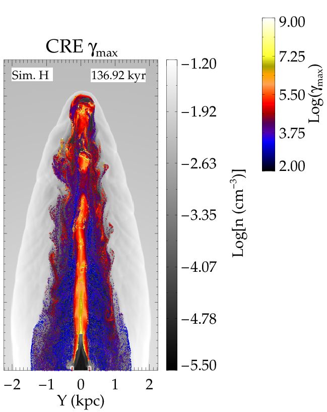
8     Mukherjee et al.

                                                                                                  Sim. B
                                                                              7                                      20
                                                                              6
                                                                                                                     15

                                                                                                                         Number of shocks
                                                                              5
                                                                                      P1
                                                                              4

                                                                    z [kpc]
                                                                                                                     10
                                                                              3              P3
                                                                              2                                      5
                                                                                                       P2 P4
                                                                              1                                      1

                                                                                  1
                                                                                  y[ 0                          1
                                                                                    kp                 0
                                                                                      c] 1
                                                                                                  1         ]
                                                                                                      x [kpc
Figure 6. Left: Density slice in the X − Z plane for simulation B with log(γmax ) of CREs over-plotted, similar to the lower panel of
Fig. 5. Right: Tracks of 4 representative particles, as also presented in Fig. 4.

with a steady magnetic field fluctuating about a mean of             correlates with an increase in the compression ratio, indicat-
∼ 0.04 mG. The γmax shows some initial increase as the CRE           ing that the particles have traversed through strong shocks
travels through the jet-axis and reaches the complex shock at        with compression ratios r >∼ 2 − 4. The multiple peaks in the
the jet-head, as also corroborated from the initial changes in       γmax at different times result from re-acceleration at internal
compression ratio. However, post jet exit, the CRE streams           shocks during their motion within the cocoon. The low mean
through the backflow with an exponential decay of γmax . The         injected magnetic field in this simulation, also contribute to
evolution of P2 is thus along the lines of the standard expec-       the high values of γmax .
tation of CRE evolution proposed in traditional analytical              • Simulation H: For simulation H, we present the results
models (Jaffe & Perola 1973; Turner & Shabala 2015), as              for 3 CREs. CRE P1 exits the jet at Z ∼ 3 kpc and proceeds
also depicted in Fig. 3. However, CRE P3 with multiple shock         laterally onwards into the cocoon. CREs P3 and P4 injected
crossings spread over a long duration, is a result of the local      at later times exit at a higher height (Z ∼ 9 kpc). As CRE
inhomogeneities due to non-linear MHD.                               P1 proceeds through the jet axis, it experiences an initial
   Another point to note is that, the high γmax of CRE P3            rise of magnetic field along its trajectory, followed by a lower
coincide with high values of the compression ratio (r > 1.5).        value of ∼ 0.1 mG. CREs P3 and P4 having been injected at
This is expected, as strong shocks of higher compression ra-         similar times, follow similar trajectories and show a similar
tio (r), will give rise to higher values of γmax for the same        nature of the time evolution of the magnetic field and shock
strength of magnetic field, as can be seen in Eq. (A8) and           compression ratio. The initial γmax of P3 is higher as it likely
Eq. (A9). However, for CRE P2, the initial rise in γmax cor-         passes through a stronger recollimation shock after injection,
responds to crossings of weak shock (r < ∼ 1.3), and also lower      than P4.
magnetic field strengths than P3 by nearly an order of mag-             Although the CREs experience stronger shocks than simu-
nitude. As can again been seen from Eq. (A8), lower values           lation D, the γmax is not much higher than that in simulation
of magnetic field strength at shocks will also result in an in-      D. The stronger magnetic field in simulation H, causes faster
crease in γmax due to lower synchrotron cooling times. Thus          radiative losses of the CREs reducing the efficiency of shock
these two CREs demonstrate well how CREs can experience              acceleration.
different physical conditions during their trajectory, and how
they differently affect their spectra.
                                                                     5.3 Multiple internal shocks
   • Simulation D: For simulation D (middle column of
Fig. 9), we present the results for CREs P1 and P2 labelled in       As stated earlier in previous sections, MHD instabilities cre-
Fig. 8, which have very different spatial tracks, as discussed       ate complex shock structures inside the jet cocoon where
earlier in Sec. 5.1.2. The turbulent magnetic field fluctuating      CREs can be re-accelerated. Fig. 10 shows the probabil-
on smaller length scales than other simulations results in the       ity distribution function (hereafter PDF) of the number of
CREs experiencing a magnetic field fluctuating about a mean          shocks encountered by CREs in different simulations. Simu-
value (∼ 0.04 mG) as well. The γmax however shows sharp              lations with similar power are plotted with same linestyles
increase followed by phases of decline. The increase in γmax         although different colours viz. simulations D (green) and F

MNRAS 000, ??–?? (2015)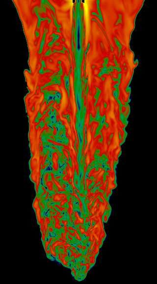
Evolution of non-thermal electrons                  9
                                                                       of bi-modality. This results from joint contributions of the
                                                                       CREs in the jet spine which are shocked only at a few recol-
                                                                       limation shocks and the CREs in the cocoon which have been
                                    Extended shock                     shocked many times at the jet head or the internal shocks in
                                    structure due to                   the cocoon.
                                     bent jet-head
                                                                       5.4 Maximum Lorentz factor of CREs
                                                                       5.4.1 Distribution of γmax at different heights
                                                                       In this section we discuss the effect of multiple shock encoun-
                                                                       ters on the maximum Lorentz factor of the CREs (γmax ),
                                                                       which is defined by Eq. (A8). Fig. 11 shows the PDF of the
                                                                       γmax at three different heights, corresponding to the jet-head
                                                                       (∼ 7 kpc, in blue), the middle zone (∼ 5 kpc, in brown)
  Recollimation                                                        and the base of the cocoon (∼ 3 kpc, in black), for different
  shocks in jet                                                        simulations. The PDFs at different heights are instructive to
     spine                                                             understand the evolution of the CRE spectra, as they are
                                                                       shocked at the jet-head and later again while crossing weaker
                                                                       shocks in the back-flow.
                                                                          Firstly, it is evident that the PDFs have a more extended
                                                                       distribution (γmax ∼ 109 ) closer to the jet head (∼ 7 kpc),
                                                                       where they encounter the strong terminal shock. The PDFs
                                                                       in the mid-planes for simulation B have a lower value of max-
                                                                                                         8
                                                                       imum Lorentz factor (γmax <   ∼ 10 ) as they consist of particles
                                                                       that have cooled due to radiative losses. However, in sim-
                                                                       ulations D and G, γmax in the middle zone extends up to
                                                                       γmax ∼ 109 as particles get re-accelerated by internal shocks
                                                                       inside the cocoon.
                                                                          The PDFs have a general nature of a peak at γmax ∼ 105 ,
                                                                       followed by an extended tail. The peak and the lower end
                                                                       of the PDF is often well described by a log-normal distribu-
               Shocks in                                               tion, as shown by the dotted lines in Fig. 11. The peak of
                cocoon                                                 the lognormal shows a decreasing trend with distance from
                                                                       the jet-head, indicating radiative losses. The tail of the PDF
                                                                       extending beyond the log-normal to high Lorentz factors
                                                                       (γmax ∼ 108 − 109 ), comprises of freshly shocked electrons.
             Recollimation                                             Such particles thus form a different population of highly en-
                shocks                                                 ergetic, freshly shocked electrons. The PDF at ∼ 7 kpc for
                                                                       simulation F (middle panel, in red) indeed shows a bi-modal
                                                                       distribution with the higher peak also described by a log-
                                                                       normal like distribution.

                                                                       5.4.2 Multiple shocked components
                                                                       The onset of MHD instabilities creates different population of
                                                                       CREs with different shock histories and energetics. This can
                                                                       be seen from the 2D PDFs of the number of shock crossings of
Figure 7. A 3D volume rendering of shocked surfaces in the co-         the CREs and the γmax in Fig. 12. The PDFs have been made
coon of simulation B (top) and simulation D (bottom). The shocks       at a height of z = 5 ± 0.2 kpc, which is approximately half
are identified by the ∆p/p > 3, as described in Sec. 5.1.2. The spa-   the jet-height at the end of the simulation. The half height
tial scale of the axes are in kilo-parsecs.                            was selected so that CREs have enough time to settle into
                                                                       the backflow inside the cocoon, after exiting jet.
                                                                         We can see that in general three zones can be identified,
(brown) with Pjet ∼ 1045 erg s−1 in dashed, and simula-
                                                                       for three different populations of CREs:
tions G (blue) and H (red) with Pjet ∼ 1046 erg s−1 in solid.
Kelvin-Helmholtz instabilities in simulation D result in higher           • Pop. I: They are represented approximately by the black-
number of shock crossing with the PDF showing a very ex-               box in dash-dotted contours, over-plotted on the PDF maps
tended tail than that in others. Similarly, simulation G which         in Fig. 12. Such CREs have experienced 5-10 shock crossing
has more internal structures and shocks due to higher inter-           (lower for simulation B) and have γmax ∼ 104 − 106 , peaking
nal sound speed has a slightly extended PDF than the stable            around γmax ∼ 105 . This is typical for CREs whose higher
jet in simulation H. Simulations F and H show a slight hint            energy part of the spectra is decaying due to radiative losses.

                                                                                                            MNRAS 000, ??–?? (2015)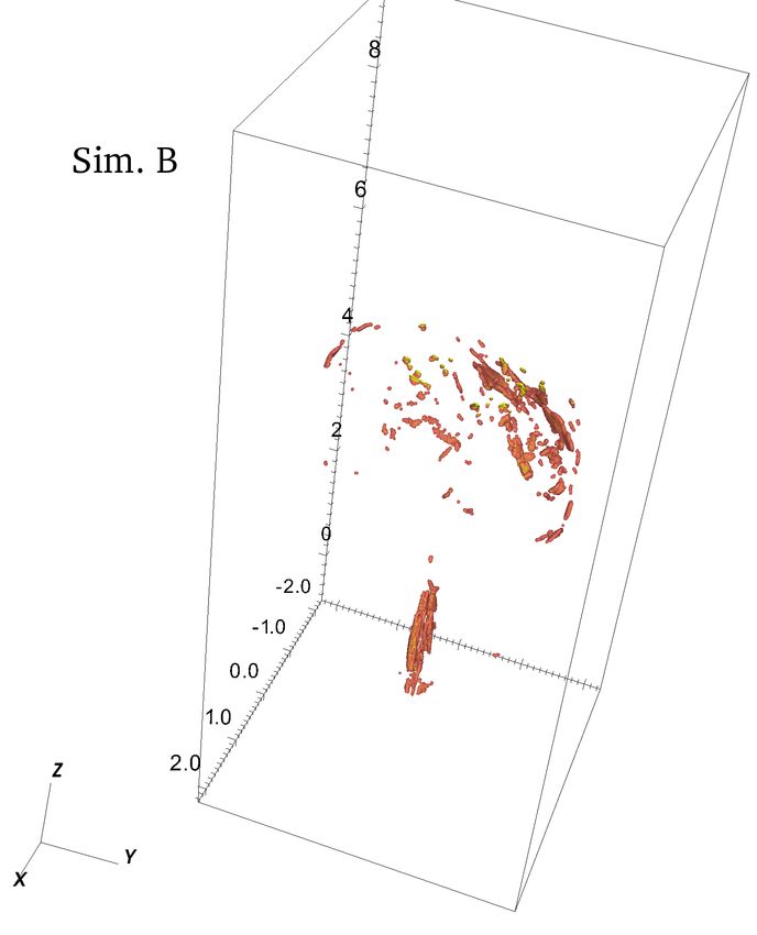
10 Mukherjee et al.
Sim. D
9
P2 20
8
7 15
Number of shocks
6
5 10
z [kpc]
4
3 5
P1
2
1
1
1
y [k 0 0 1
pc] 11
x [kpc]
Figure 8. Left: Tracks of two representative CREs in simulation D. The track of P1 is shown by a red-line connecting its locations at
different times. Similarly, the track of CRE P2 is represented by the blue line connecting the dots. The color of the dots denotes the
number of shock crossings experienced (as also in Fig. 4). Middle: The density slice for simulation D with particle color showing age since
last shock, as in the lower panel of Fig. 5. Right: Density slice, with particle color showing log(γmax ), as in the upper panel of Fig. 5. A
larger portion of the cocoon has freshly shocked particles due to turbulence generated shocks in the cocoon depicted in the left panel.
Magnetic field traced by particles Magnetic field traced by particles Magnetic field traced by particles
0.200 Sim. B 0.10 Sim. D 2.00 Sim. H
Magnetic field [mG]
0.175
Magnetic field [mG]
P1
Magnetic field [mG]
P2 P1 1.75
0.150 0.08 P2 P3
P3 1.50 P4
0.125 0.06 1.25
0.100 1.00
0.075 0.04 0.75
0.050 0.02 0.50
0.025 0.25
0.00 0.00
600 650 700 750 800 850 900 950 150 200 250 300 350 400 450 40 60 80 100 120 140 160 180
Time [kyr] Time [kyr] Time [kyr]
Maximum Lorentz factor Maximum Lorentz factor 9
Maximum Lorentz factor
8.0 Sim. B 9.0 Sim. D Sim. H
7.5 8.5 8 P1
P2 P1 P3
7.0 P3 8.0 P2 P4
7
max)
max)
max)
7.5
6.5 7.0 6
Log (
Log (
Log (
6.0 6.5
5.5 6.0 5
5.0 5.5 4
5.0
600 650 700 750 800 850 900 950 150 200 250 300 350 400 450 40 60 80 100 120 140 160 180 200
Time [kyr] Time [kyr] Time [kyr]
Compression ratio since last shock 6Compression ratio since last shock Compression ratio since last shock
Sim. B Sim. D 14 Sim. H
3.5
Compression ratio
5 P1 12 P1
Compression ratio
Compression ratio
P2 P3
3.0 P3 P2 10
4 P4
2.5 8
3 6
2.0 4
1.5 2 2
1 0
600 650 700 750 800 850 900 950 150 200 250 300 350 400 450 40 60 80 100 120 140 160 180
Time [kyr] Time [kyr] Time [kyr]
Figure 9. The magnetic field (top row), maximum Lorentz factor (middle row) and shock compression ratio since last shock (last panel
row) traced by some CREs, whose trajectories are presented in Fig. 6, Fig. 8 and Fig. 4 for simulations B (left column), D (middle column)
and H (right column) respectively.
MNRAS 000, ??–?? (2015)Evolution of non-thermal electrons 11
PDF of number of shocks crossed particles within the jet-spine and the cocoon. The above has
been performed for simulations D and F, at the end of the
0.1000 Sim. B
Sim. D respective simulations, when the jet has reached a height of
Sim. F ∼ 9 kpc, such that the height chosen to extract the CREs
Sim. G
Sim. H approximately represents the middle of the jet-cocoon struc-
ture.
dN/NTotal
0.0100
We firstly notice a bi-modal distribution, with the lower
values in the green box representing CREs inside the jet.
These CREs have been recently injected, and hence the low
0.0010 age. They travel at near light-speed up to a height of ∼ 5 kpc,
as can be seen from the green horizontal lines in the figures,
showing tage = 5 kpc/(cTsim ), where Tsim is the end time of
the simulation. The above line represents the lower-end of the
0.0001
0 5 10 15 20
distribution, with the rest of the particles being older owing
Number of shocks to slower propagation speed inside the jet-axis.
Above the CREs in the jet beam, there is an extended
Figure 10. The distribution of number of shocks traversed by the distribution of CREs, which represent the CREs inside the
particles during their lifetime for simulations B, D, F, G and H. cocoon.The cocoon CREs at ∼ 5 kpc cover wide range in
Stable jets in F and H have steep tail due to lower shock crossings.
ages, demarcated by the two limits, tL and tU respectively,
Simulation D with Kelvin-Helmholtz modes has an extended tail
as denoted in the figure. The upper limit, tU , from the old-
indicating many crossings.
est CREs at Z = 5 kpc, correspond to particles that have
exited the jet spine when the jet-head had reached a height
The mean spread of γmax of these CREs corresponds well of ∼ 5 kpc during its evolution, and have remained at the
with the peak of the log-normal distribution at ∼ 5 kpc in similar height up to the end of the simulation. In the regular
Fig. 11 discusses earlier. Thus these CREs represent the bulk back-flow model, one would expect the CREs to then stream
of the non-thermal electrons in the cocoon whose spectrum downwards into the cocoon. However, several CREs follow
follow the standard evolutionary scenario of being accelerated complex trajectories, which are often lateral, as also shown
at the jet-head and followed by radiative cooling, as shown in Fig. 6 and Fig. 8. These CREs hover around the original
in the cartoon in Fig. 3. height from which they had exited the jet, which likely result
• Pop. II: There is a second population of CREs, especially from internal turbulent flows. Being older, they also have a
7
for simulation D and F, with high energies (γmax ∼ 107 − lower value of γmax < ∼ 10 , due to radiative losses. The lower
109 ), but less number of shock crossings (Nshock ∼ 2 − 5). limit, tL , correspond to CREs that have exited the jet at a
They are highlighted by a green box with dashed contours more recent time, when the jet has evolved to a larger height,
in the middle and right panels of Fig. 12. These are CREs and subsequently travelled downwards to Z ∼ 5 kpc with the
in the jet spine, which have been energised by recollimation backflow.
shocks, and hence the high γmax . Since, there are only a few The above age ranges can be better understood by con-
of recollimation shocks in the jet, they have undergone only structing an approximate model of the time spent by a CRE
a handful of shock-crossings. from its injection to its final position in a backflow. Suppose
• Pop. III: A third population of CREs can be identified in the CRE after injection at the base of the jet, travels along
simulations B and D, which have high γmax ∼ 107 − 109 and along the flow with a mean propagation speed vj , and exits
multiple shock crossings (Nshock > 5), denoted by the orange the main jet-flow at a height Z ∗ at a time t∗ after encounter-
box in the left and middle figures of the top panel in Fig. 12. ing the jet-head. The CRE then must have been injected into
These CRE have crossed multiple shocks either in the com- the jet-stream at an earlier time tinj = t∗ − (Z ∗ /vj ), where
plex structure at the jet-head (as in simulation B) or internal Z ∗ /vj denotes the travel time within the jet-axis. Then if the
shocks inside the cocoon (e.g. simulation D). This is a signa- end of the simulation (or in other words the current age of
ture of jets with active MHD instabilities, and is distinctly the jet) is Tsim , the age of the CRE will be:
absent in simulation F, which is stable to both kink and KH
modes, as also reported recently in Borse et al. (2020). In sim- tage = Tsim − tinj = Tsim − (t∗ − (Z ∗ /vj )) . (12)
ulation F, after crossing the jet-head, the CREs cool down in After exiting the jet, the CRE freely streams down along a
the backflow, without being re-accelerated, unlike the CREs regular backflow. If the mean backflow velocity is vb , then
in Pop. III category. for a CRE at a height L in the backflow (measured from the
central source):
5.5 Distribution of CRE ages at a given height
vb (T − t∗ ) = Z ∗ − L (13)
The cocoon has a wide distribution of CRE ages due to their
different propagation history. This is accentuated in a tur- If we assume the mean propagation speed of the jet-head to
bulent jet where regular streamlines inside the backflow are be vh , such that t∗ = Z ∗ /vh , then combining Eq. (12) and
disrupted due to instabilities. In Fig. 13 we present the 2D Eq. (13) to eliminate Z ∗ , we get
distribution of γmax and the CRE age since injection into
L (vj − vh ) vb
the computational domain, normalised by the simulation run- tage = T − T + (14)
vb (vb + vh ) vj
time. The PDFs have been constructed by extracting all par-
ticles at a height of Z = 5 ± 0.2 kpc, which includes both Eq (12)–(14) together give an approximate estimate of the
MNRAS 000, ??–?? (2015)12 Mukherjee et al.
Maximum γe
0.1000 G: 3 kpc
44 −1
P=10 ergs B: 3 kpc P=10 ergs−1
45
D: 3 kpc P=1046 ergs−1 G: 5 kpc
B: 5 kpc D: 5 kpc
G: 7 kpc
B: 7 kpc D: 7 kpc
H: 7 kpc
F : 7 kpc
0.0100
dN/N
0.0010
0.0001
3 4 5 6 7 8 9 4 5 6 7 8 9 10 2 3 4 5 6 7 8 9
Log(γe)
Figure 11. The distribution of γ for different simulations, at three different heights, following the convention of Fig. 10. The three panels
correspond to simulations of in 3 ranges of power. The PDFs in general show a peak (which is well described by a log-normal distribution
shown in dashed lines), followed by an extended tail to high γ.
Figure 12. 2D PDF of γmax vs number of shocks crossed (Nshock ) by a CRE macro-particle at a height z = 5 kpc at the end of the
simulation. Three different CRE populations have been highlighted in coloured boxes. 1) Pop. I in the black box: Older CREs with
decayed spectra. 2) Pop. II in green box: Freshly shocked CREs with high energies that lie in the jet spine. 3) Pop. III in orange box:
re-accelerated CREs that have been shocked many times.
Distribution of Zmax
0.7
Normalised histogram
0.6 Sim. F, tage L
0.5 Sim. F, tage U
Sim. D, tage L
0.4 Sim. D, tage U
0.3
0.2
0.1
0.0
5.0 5.5 6.0 6.5 7.0 7.5 8.0 8.5
Zmax
Figure 13. Left & Middle: 2D PDF of γmax vs time elapsed since a CRE is injected (tage ) representing the age of a CRE in the
simulation, normalised to the total simulation time (Tsim ). The green box denotes CREs inside the jet. The green dashed line denotes
the time to reach z = 5 kpc with a speed c, normalised to the simulation time. The blue lines, marked by tL and tU denote the extent
of the distribution of ages within the cocoon that have exited the jet. See text in Sec. 5.5 for further details. Right: The distribution of
maximum height (Zmax ) reached by particles with the ages tL and tU in the previous panels.
MNRAS 000, ??–?? (2015)Evolution of non-thermal electrons 13
Spectral evolution of a particle
Vz Vz 109
104 Sim. D
Normalised spectra
0.50
Sim. D 391.18 kyr Sim. F 234.71 kyr
8 10 1
0.33
10 6
6 0.17 10 11
Nshock: 2, t: 71 kyr
10 16 Nshock: 9, t: 81 kyr
Z [kpc]
Vz/c
0.00 10 21 Nshock:17, t: 107 kyr
4 Nshock:20, t: 114 kyr
10 26 Nshock:22, t: 195 kyr
-0.17
100 102 104 106 108
2
-0.33
-0.50 Figure 15. The evolution of the spectra for particle P1 in sim-
-1 0 1 -1 0 1 ulation D from Fig. 8. The legends show the number of shocks
Y [kpc] Y [kpc] crossed and the simulation time for each spectrum. The spectra
are normalised to their maximum value. Each spectrum is offset
vertically by a factor of 100 from the one below for better visual
representation.
Figure 14. The vz component of the velocity field (normalised
to c) for simulations D and F. Simulation F shows an extended
backflow that remains mildly relativistic (∼ 0.3 − 0.5c) for a major tion of maximum heights reached by CREs with tage = tL for
part of the cocoon. For simulation D, the backflow loses momentum
simulations D and F, as shown in the right panel of Fig. 13.
after a few kpc from the current location of the jet-head.
While simulation F has a sharp peak at Zmax ∼ 7 kpc, simi-
lar CREs in simulation D has a broader distribution, ranging
between ∼ 6−8 kpc. This points to the fact that simulation F
Table 2. Estimates of tU from Eq. (12)
being stable to MHD instabilities, has a regular, well-defined
backflow, as can also be seen in Fig. 14. However, MHD in-
Sim. t∗ Tsim vj /c tage /Tsim
stabilities in simulation D disrupt the backflow resulting in
label (kyr) (kyr)
intermittent flow patterns and mean speed for different CRE
D 205 391 0.35 0.6 stream-lines. This results in a wider distribution of CREs of
F 166 235 0.7 0.39 different ages at a given height.
time taken by the CRE to reach a certain height in the back- 5.6 Evolution of CRE spectrum
flow. For CREs at tU , Z∗ = 5 kpc, and t∗ is the time at which
5.6.1 Spectrum as a function of time for a single CRE
the jet reached a height of ∼ 5 kpc. Using approximate es-
timates of mean advance speed within the jet vj , one gets The spectrum of a CRE macro-particle changes in the simu-
approximate estimates of tage which well match with Fig. 13, lation due to two reasons: i) shock encounters that accelerate
as shown in Table 2. Note a lower value of propagation speed the electrons and ii) radiative losses due to synchrotron or
of the CRE is used for simulation D. This results from the inverse-Compton emission. Losses due to inverse-Compton
deceleration of the jet-head due to Kelvin-Helmholtz insta- interaction with CMB are nearly constant at all locations,
bilities, resulting in a slower mean propagation speed of the and secondary to synchrotron driven cooling for strong mag-
CRE inside the jet axis. netic fields (B >
∼ BCMB , as in Ghisellini et al. 2014). For the
Similarly, to model the ages of the CREs at tL , assum- simulations explored in this work, the magnetic field is well
ing (vj , vb , vh ) ≡ (0.9, 0.3, 0.065)c for simulation D, gives above the critical field. Fig. 15 shows the evolution of the
tage ∼ 0.13Tsim , for the chosen height of L = 5 kpc. This spectrum of particle P1 of simulations D whose trajectory
is close to the observed limit in Fig. 13. Similarly, for sim- has been shown in Fig. 8. The figures show how the spectrum
ulation F, the choice of (vj , vb , vh ) ≡ (0.9, 0.3, 0.1)c gives changes after the particle has experienced multiple shock en-
tage ∼ 0.18Tsim . The above choices though adhoc, are rea- counters.
sonable in their values and are indicative of the nature of the At the initial stages the spectra are well represented by a
CRE motion in the backflow. In Fig. 14 we show the Z com- power-law with a sharp cut off due to cooling losses, as ex-
ponent of the velocity, depicting the velocity in the jet as well pected from a cooling population of shocked electrons (Har-
as the backflow. It can be seen that the choice of vj ∼ 0.9c wood et al. 2013). However, the energy distributions at the
and vb ∼ 0.3c are within limits of the actual values inferred intermediate times are not described by a simple power-law
from the velocity maps in Fig. 14. A smaller value of vh is with an exponential cut-off. Some of the spectra have a curved
used for simulation D to account for the decelerated jet ad- shape, well approximated by piece-wise power-laws (for ex-
vance due to Kelvin-Helmholtz instabilities. The value used is ample the red and green curves). Such an evolution may arise
consistent with the mean advance speed of the jet presented when multiple shocks of varying strengths are encountered,
in Fig 15 of Mukherjee et al. (2020). as was demonstrated in the top panel of Fig. 1, in Sec. 2.1.2.
An interesting point to note is the nature of the distribu- However, the high energy tail will eventually decay with time
MNRAS 000, ??–?? (2015)You can also read