Skin CSE169: Computer Animation Instructor: Steve Rotenberg UCSD, Winter 2020 - UCSD CSE

Skin
CSE169: Computer Animation
 Instructor: Steve Rotenberg
 UCSD, Winter 2020

Rendering Review

Rendering
◼ Renderable surfaces are built up from
 simple primitives such as triangles
◼ They can also use smooth surfaces such
 as NURBS or subdivision surfaces, but
 these are often just turned into triangles by
 an automatic tessellation algorithm before
 rendering

Lighting
◼ We can compute the interaction of light with
 surfaces to achieve realistic shading
◼ For lighting computations, we usually require a
 position on the surface and the normal
◼ GL does some relatively simple local illumination
 computations
◼ For higher quality images, we can compute
 global illumination, where complete light
 interaction is computed within an environment to
 achieve effects like shadows, reflections,
 caustics, and diffuse bounced light

Gouraud & Phong Shading
◼ We can use triangles to give the appearance of a
 smooth surface by faking the normals a little

◼ Gouraud shading is a technique where we compute the
 lighting at each vertex and interpolate the resulting color
 across the triangle
◼ Phong shading is more expensive and interpolates the
 normal across the triangle and recomputes the lighting
 for every pixel

Materials
◼ When an incoming beam of light hits a
 surface, some of the light will be
 absorbed, and some will scatter in various
 directions

Materials
◼ In high quality rendering, we use a function
 called a BRDF (bidirectional reflectance
 distribution function) to represent the scattering
 of light at the surface:

 fr(θi, φi, θr, φr, λ)

◼ The BRDF is a 5 dimensional function of the
 incoming light direction (2 dimensions), the
 outgoing direction (2 dimensions), and the
 wavelength

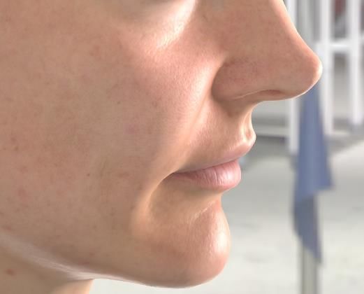
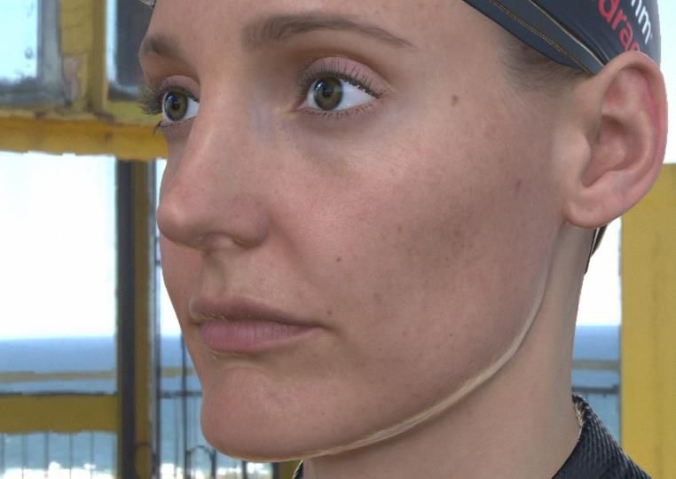
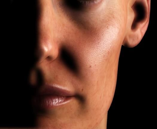
Translucency
◼ Skin is a translucent material. If we want to
 render skin realistically, we need to account for
 subsurface light scattering.
◼ We can extend the BRDF to a BSSRDF by
 adding two more dimensions representing the
 translation in surface coordinates. This way, we
 can account for light that enters the surface at
 one location and leaves at another.
◼ Learn more about these in CSE168!

Texture
◼ We may wish to ‘map’ various properties across the
 polygonal surface
◼ We can do this through texture mapping, or other more
 general mapping techniques
◼ Usually, this will require explicitly storing texture
 coordinate information at the vertices
◼ For higher quality rendering, we may combine several
 different maps in complex ways, each with their own
 mapping coordinates
◼ Related features include bump mapping, displacement
 mapping, illumination mapping…

Skin Rendering

Position vs. Direction Vectors
◼ We will almost always treat vectors as having 3
 coordinates (x, y, and z)
◼ However, when we actually transform them by a 4x4
 matrix, we expand them to 4 coordinates
◼ Vectors representing a position in 3D space are
 expanded into 4D as:

 v x vy vz 1 
◼ Vectors representing direction (like a normal or an axis
 of rotation) are expanded as:

 v x vy vz 0 

Position Transformation
 v = M  v
vx   a1 b1 c1 d1  v x 
 v    a b c d  v 
 y =  2 2 2 2  y
 
 vz   a3 b3 c3 d 3   vz 
     
1 0 0 0 1  1
vx = a1v x + b1v y + c1v z + d1
vy = a2 v x + b2 v y + c2 vz + d 2
vz = a3v x + b3v y + c3v z + d 3
1 = 0v x + 0v y + 0vz + 1

Direction Transformation

Smooth Skin Algorithm

Weighted Blending & Averaging
◼ Weighted sum: x =  wi xi
 i =0

◼ Weighted average: w
 i =0
 i =1

◼ Convex average: 0  wi  1

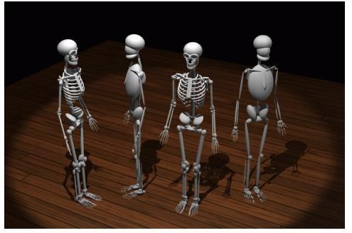
Rigid Parts
◼ Robots and mechanical creatures can usually
 be rendered with rigid parts and don’t require a
 smooth skin
◼ To render rigid parts, each part is transformed
 by its joint matrix independently
◼ In this situation, every vertex of the character’s
 geometry is transformed by exactly one matrix

 v = W  v
 where v is defined in joint’s local space

Simple Skin
◼ A simple improvement for low-medium quality
 characters is to rigidly bind a skin to the
 skeleton. This means that every vertex of the
 continuous skin mesh is attached to a joint.
◼ In this method, as with rigid parts, every vertex
 is transformed exactly once and should
 therefore have similar performance to rendering
 with rigid parts.

 v = W  v

Smooth Skin
◼ With the smooth skin algorithm, a vertex can be
 attached to more than one joint with adjustable
 weights that control how much each joint affects
 it
◼ Verts rarely need to be attached to more than
 three joints
◼ Each vertex is transformed a few times and the
 results are blended
◼ The smooth skin algorithm has many other
 names: blended skin, skeletal subspace
 deformation (SSD), multi-matrix skin, matrix
 palette skinning…

Smooth Skin Algorithm
◼ The deformed vertex position is a
 weighted average:
 v = w1 (M1  v ) + w2 (M 2  v ) + ...wN (M N  v )
 or
 v =  wi (M i  v )
 where
 w i =1

Binding Matrices
◼ With rigid parts or simple skin, v can be defined local to
 the joint that transforms it
◼ With smooth skin, several joints transform a vertex, but it
 can’t be defined local to all of them
◼ Instead, we must first transform it to be local to the joint
 that will then transform it to the world
◼ To do this, we use a binding matrix B for each joint that
 defines where the joint was when the skin was attached
 and premultiply its inverse with the world matrix:
 −1
 M i = Wi  B i

Binding Matrices
◼ Let’s look closer at this:

 ′ = ⋅ −1 ⋅ 

◼ is the world matrix that joint i had at the time the skeleton was
 matched to the skin (the binding pose)
◼ transforms verts from a space local to joint i into this binding pose
◼ Therefore, −1 transforms verts from the binding pose into joint i
 local space
◼ transforms from joint I local space to world space
◼ v is a vertex in the skin mesh (in the binding pose)
◼ Therefore, the entire equation transforms the vertex from the binding
 pose (v), into joint local space ( −1 ) and then into world space ( )

Normals
◼ To compute shading, we need to
 transform the normals to world space also
◼ Because the normal is a direction vector,
 we don’t want it to get the translation from
 the matrix, so we only need to multiply the
 normal by the upper 3x3 portion of the
 matrix
◼ For a normal bound to only one joint:
 n = W  n

Normals
◼ For smooth skin, we must blend the normal as
 with the positions, but the normal must then be
 renormalized:

 n =
  w (M  n )
 i i

  w (M  n )
 i i

◼ If the matrices have non-rigid transformations,
 then technically, we should use:
  w (M )
 −1T
 n
 n = i i

  w (M n)
 −1T
 i i

Algorithm Overview
Skin::Update() (view independent processing)
◼ Compute skinning matrix for each joint: M=W·B-1 (you can
 precompute and store B-1 instead of B)
◼ Loop through vertices and compute blended position & normal

Skin::Draw() (view dependent processing)
◼ Set GL matrix state to Identity (world)
◼ Loop through triangles and draw using world space positions &
 normals

Questions:
- Why not deal with B in Skeleton::Update() ?
- Why not just transform vertices within Skin::Draw() ?

Rig Data Flow

 Φ = 1  2 ...  N 
◼ Input DOFs

◼ Rigging system Rig
 (skeleton, skin…)

◼ Output renderable mesh v , n 
 (vertices, normals…)

Skeleton Forward Kinematics
◼ Every joint computes a local matrix based on its DOFs
 and any other constants necessary (joint offsets…)

 L = L jn t (1 ,  2 ,...,  N )
◼ To find the joint’s world matrix, we compute the dot
 product of the local matrix with the parent’s world matrix

 W = W p a ren t  L
◼ Normally, we would do this in a depth-first order starting
 from the root, so that we can be sure that the parent’s
 world matrix is available when its needed

Smooth Skin Algorithm
◼ The deformed vertex position is a weighted average over all of the
 joints that the vertex is attached to:

 v =  wi W i  B i  v
  −1

◼ W is a joint’s world matrix and B is a joint’s binding matrix that
 describes where it’s world matrix was when it was attached to the
 skin model (at skin creation time)
◼ Each joint transforms the vertex as if it were rigidly attached, and
 then those results are blended based on user specified weights
◼ All of the weights must add up to 1: wi = 1
◼ Blending normals is essentially the same, except we transform them
 as direction vectors (x,y,z,0) and then renormalize the results
 n*
 n * =  wi Wi  B i−1  n , n = *
 n

Skinning Equations
◼ Skeleton L = L jnt (1 , 2 ,...,  N )
 W = Wparent  L

 v =  wi Wi  B i−1  v
 n* =  wi Wi  B i−1  n
◼ Skinning *
 n
 n = *
 n

Using Skinning

Limitations of Smooth Skin
◼ Smooth skin is very simple and quite fast, but its
 quality is limited
◼ The main problems are:
 ◼ Joints tend to collapse as they bend more
 ◼ Very difficult to get specific control
 ◼ Unintuitive and difficult to edit
◼ Still, it is built in to most 3D animation packages
 and has support in both OpenGL and Direct3D
◼ If nothing else, it is a good baseline upon which
 more complex schemes can be built

Limitations of Smooth Skin

Bone Links
◼ To help with the collapsing joint problem, one
 option is to use bone links
◼ Bone links are extra joints inserted in the
 skeleton to assist with the skinning
◼ They can be automatically added based on the
 joint’s range of motion. For example, they could
 be added so as to prevent any joint from rotating
 more than 60 degrees.
◼ This is a simple approach used in some real
 time games, but doesn’t go very far in fixing the
 other problems with smooth skin.

Shape Interpolation
◼ Another extension to the smooth skinning
 algorithm is to allow the verts to be modeled at
 key values along the joints motion
◼ For an elbow, for example, one could model it
 straight, then model it fully bent
◼ These shapes are interpolated local to the
 bones before the skinning is applied
◼ We will talk more about this technique in the
 next lecture

Muscles & Other Effects
◼ One can add custom effects such as muscle
 bulges as additional joints
◼ For example, the bicep could be a translational
 or scaling joint that smoothly controls some of
 the verts in the upper arm. Its motion could be
 linked to the motion of the elbow rotation.
◼ With this approach, one can also use skin for
 muscles, fat bulges, facial expressions, and
 even simple clothing
◼ We will learn more about advanced skinning
 techniques in a later lecture

Rigging Process
◼ To rig a skinned character, one must have a geometric
 skin mesh and a skeleton
◼ Usually, the skin is built in a relatively neutral pose, often
 in a comfortable standing pose
◼ The skeleton, however, might be built in more of a zero
 pose where the joints DOFs are assumed to be 0,
 causing a very stiff, straight pose
◼ To attach the skin to the skeleton, the skeleton must first
 be posed into a binding pose
◼ Once this is done, the verts can be assigned to joints
 with appropriate weights

Skin Binding
◼ Attaching a skin to a skeleton is not a trivial
 problem and usually requires automated tools
 combined with extensive interactive tuning
◼ Binding algorithms typically involve heuristic
 approaches
◼ Some general approaches:
 ◼ Containment
 ◼ Point-to-line mapping
 ◼ Several others

Containment Binding
◼ With containment binding algorithms, the user manually
 approximates the body with volume primitives for each
 bone (cylinders, ellipsoids, spheres…)
◼ The algorithm then tests each vertex against the
 volumes and attaches it to the best fitting bone
◼ Some containment algorithms attach to only one bone
 and then use smoothing as a second pass. Others
 attach to multiple bones directly and set skin weights
◼ For a more automated version, the volumes could be
 initially set based on the bone lengths and child
 locations

Point-to-Line Mapping
◼ A simple way to attach a skin is treat each
 bone as one or more line segments and
 attach each vertex to the nearest line
 segment
◼ A bone is made from line segments
 connecting the joint pivot to the pivots of
 each child

Skin Adjustment
◼ Mesh Smoothing: A joint will first be attached in a fairly
 rigid fashion (either automatic or manually) and then the
 weights are smoothed algorithmically
◼ Rogue Removal: Automatic identification and removal of
 isolated vertex attachments
◼ Weight Painting: Some 3D tools allow visualization of the
 weights as colors (0…1 -> black…white). These can
 then be adjusted and ‘painted’ in an interactive fashion
◼ Direct Manipulation: These algorithms allow the vertex to
 be moved to a ‘correct’ position after the bone is bent,
 and automatically compute the weights necessary to get
 it there

Hardware Skinning
◼ The smooth skinning algorithm is simple and
 popular enough to have some direct support in
 3D rendering hardware
◼ Actually, it just requires standard vector
 multiply/add operations and so can be
 implemented in vertex shaders
◼ In order to make the array of matrices available
 to the shader, it may be necessary to store it in a
 special texture map…

Skin Memory Usage
◼ For each vertex, we need to store:
 ◼ Rendering data (position, normal, color, texture coords,
 tangents…)
 ◼ Skinning data (number of attachments, joint index, weight…)
◼ If we limit the character to having at most 256 bones, we
 can store a bone index as a byte
◼ If we limit the weights to 256 distinct values, we can
 store a weight as a byte (this gives us a precision of
 0.004%, which is fine)
◼ If we assume that a vertex will attach to at most 4 bones,
 then we can compress the skinning data to (1+1)*4 =8
 bytes per vertex (64 bits)
◼ In fact, we can even squeeze another 8 bits out of that
 by not storing the final weight, since
 w3 = 1 – w0 – w1 – w2

Project 2: Skin

Assignment:
◼ Load a .skin file and attach it to the skeleton using the
 world space matrices to transform the positions and
 normals with the smooth skin algorithm
◼ Use basic lighting to display the skin shaded (use at
 least two different colored lights)
◼ Add some sort of interactive control for selecting and
 adjusting DOFs (can be a simple ‘next DOF’ key and
 ‘increase’ and ‘decrease’ key). The name and value of
 the DOF must be displayed somewhere
◼ Due Thursday, January 31, by 4:50 pm

Skin File
positions [num] {
 [x] [y] [z]
}
normals [num] {
 [x] [y] [z]
}
skinweights [num] {
 [numbinds] [joint0] [weight0] [j1] [w1] … [jN-1] [wN-1]
}
triangles [num] {
 [index0] [index1] [index2]
}
bindings [num] {
 matrix {
 [ax] [ay] [az] [bx] [by] [bz] [cx] [cy] [cz] [dx] [dy] [dz]
 }
}

Suggestions
◼ You might consider making classes for:
 ◼ Vertex
 ◼ Triangle
 ◼ Skin
◼ Keep a clean interface between the skin and the
 skeleton. A Skeleton::GetWorldMatrix(int) function may
 be all that is necessary. This way, the skeleton doesn’t
 need to know anything about skin and the skin only
 needs to be able to grab matrices from the skeleton.
◼ Make sure that your skeleton creates the tree in the
 correct order for the joint indexing to work correctly.

Advanced Skinning

Free-Form Deformations

Global Deformations
◼ A global deformation takes a point in 3D space and
 outputs a deformed point

 x’=F(x)

◼ A global deformation is essentially a deformation of
 space
◼ Smooth skinning is technically not a global deformation,
 as the same position in the initial space could end up
 transforming to different locations in deformed space

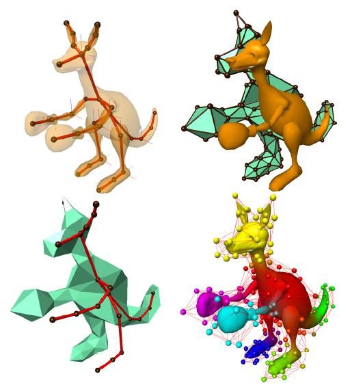
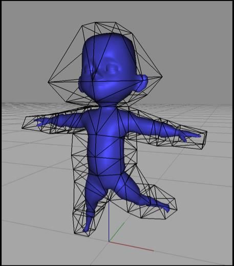
Free-Form Deformations
◼ FFDs are a class of deformations where a
 low detail control mesh is used to deform
 a higher detail skin
◼ Generally, FFDs are classified as global
 deformations, as they describe a mapping
 into a deformed space
◼ There are a lot of variations on FFDs
 based on the topology of the control mesh

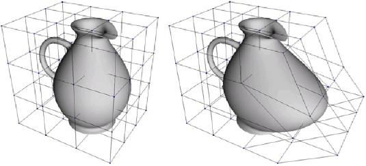
Lattice FFDs
◼ The original type of FFD uses a simple regular
 lattice placed around a region of space
◼ The lattice is divided up into a regular grid
 (4x4x4 points for a cubic deformation)
◼ When the lattice points are then moved, they
 describe smooth deformation in their vicinity

Arbitrary Topology FFDs
◼ The concept of FFDs was later extended to
 allow an arbitrary topology control volume to be
 used

Axial Deformations & WIRES
◼ Another type of deformation allows the
 user to place lines or curves within a skin
◼ When the lines or curves are moved, they
 distort the space around them
◼ Multiple lines & curves can be placed near
 each other and will properly interact

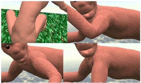
Surface Oriented FFDs
◼ This modern method allows a low detail polygonal mesh
 to be built near the high detail skin
◼ Movement of the low detail mesh deforms space nearby
◼ This method is nice, as it gives a similar type of control
 that one gets from high order surfaces (subdivision
 surfaces & NURBS) without any topological constraints

Surface Oriented FFDs

Using FFDs
◼ FFDs provide a high level control for
 deforming detailed geometry
◼ Still, we must address the issue of how to
 animate and deform the FFD control mesh
◼ The verts in the mesh can be animated
 with the smooth skinning algorithm, shape
 interpolation, or other methods

Body Scanning

Body Scanning
◼ Data input has become an important issue for
 the various types of data used in computer
 graphics
◼ Examples:
 ◼ Geometry: Laser scanners
 ◼ Motion: Optical motion capture
 ◼ Materials: Gonioreflectometer
 ◼ Faces: Computer vision
◼ Recently, people have been researching
 techniques for directly scanning human bodies
 and skin deformations

Body Scanning
◼ Practical approaches tend to use either a 3D
 model scanner (like a laser) or a 2D image
 based approach (computer vision)
◼ The skin is scanned at various key poses and
 some sort of 3D model is constructed
◼ Some techniques attempt to fit this back onto a
 standardized mesh, so that all poses share the
 same topology. This is difficult, but it makes the
 interpolation process much easier.
◼ Other techniques interpolate between different
 topologies. This is difficult also.

Body Scanning

Body Scanning

Anatomical Modeling

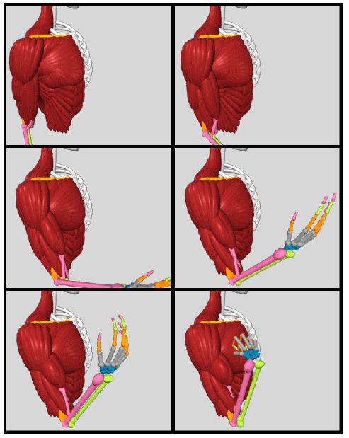
Anatomical Modeling
◼ The motion of the skin is based on the motion of
 the underlying muscle and bones. Therefore, in
 an anatomical simulation, the tissue beneath the
 skin must be accounted for
◼ One can model the bones, muscle, and skin
 tissue as deformable bodies and then then use
 physical simulation to compute their motion
◼ Various approaches exist ranging from simple
 approximations using basic primitives to detailed
 anatomical simulations

Skin & Muscle Simulation
◼ Bones are essentially rigid
◼ Muscles occupy almost all of the space between
 bone & skin
◼ Although they can change shape, muscles have
 essentially constant volume
◼ The rest of the space between the bone & skin
 is filled with fat & connective tissues
◼ Skin is connected to fatty tissue and can usually
 slide freely over muscle
◼ Skin is anisotropic as wrinkles tend to have
 specific orientations

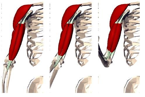
Simple Anatomical Models
◼ Some simplified anatomical models use
 ellipsoids to model bones and muscles

Simple Anatomical Models
◼ Muscles are attached to bones, sometimes with
 tendons as well
◼ The muscles contract in a volume preserving
 way, thus getting wider as they get shorter

Simple Anatomical Models
◼ Complex musculature
 can be built up from lots
 of simple primitives

Simple Anatomical Models
◼ Skin can be attached to the muscles with
 springs/dampers and physically simulated
 with collisions against bone & muscle

Detailed Anatomical Models
◼ One can also do detailed simulations that
 accurately model bone & muscle
 geometry, as well as physical properties
◼ This is becoming an increasing popular
 approach, but requires extensive set up

Detailed Anatomical Models