The vibration of a large ring-stiffened prolate dome under external water pressure
←
→
Page content transcription
If your browser does not render page correctly, please read the page content below
Ocean Engineering 31 (2004) 1–19
                                                                     www.elsevier.com/locate/oceaneng

     The vibration of a large ring-stiffened prolate
         dome under external water pressure
           Carl T.F. Ross , Andrew P.F. Little, Colin Bartlett
            Department of Mechanical Engineering, University of Portsmouth, Portsmouth, UK
        Received 6 December 2002; received in revised form 27 March 2003; accepted 25 May 2003

Abstract

  The paper presents a theoretical and an experimental investigation into the free vibration
of a large ring-stiffened prolate dome in air and under external water pressure.
  The theoretical investigation was via the finite element method where a solid fluid mesh
with an isoparametric cross-section was used to model the water surrounding the dome, and
a truncated conical shell and ring stiffener were used to model the structure. Good agree-
ment was found between theory and experiment. Both the theory and the experiment found
that as the external water pressure was increased the resonant frequencies decreased.
# 2003 Elsevier Ltd. All rights reserved.

Keywords: Vibration; Water pressure; Finite elements; Ring-stiffeners; Dome; Submarine

1. Introduction

   Some three-fourth of the Earth’s surface is covered by water and only about 1%
of the bottoms of the Earth’s oceans have been explored by man. It is the authors’
belief that during the 21st century, man’s interest in the ocean bottoms will
increase, both for military and commercial purposes. In this context, a better
understanding of the behaviour of the submarine structure will be of paramount
value. A typical submarine pressure hull consists of a combination of cylinders,
cones and domes, as shown in Fig. 1.
   It should be noted in Fig. 1, that the casing which has been put there for hydro-
dynamic reasons, surrounds the pressure hull. The casing has water on the inside
and outside surfaces and because of this, it is in a state of hydrostatic stress and it
is unlikely to fail due to hydrostatic pressure. It should also be noted from Fig. 1


     Corresponding author. Tel.: +44 23 9225 9304; fax: +44 23 9279 1129.

0029-8018/$ - see front matter # 2003 Elsevier Ltd. All rights reserved.
doi:10.1016/S0029-8018(03)00105-7
2                       C.T.F. Ross et al. / Ocean Engineering 31 (2004) 1–19

    Nomenclature

    List of   symbols
    [B]        a matrix relating strain to displacement,
                                            p              i.e. feg ¼ ½BfUi g
    c          speed of sound in water ¼ ðK=qF Þ, or c ¼ cos a
    [Cv]       matrix of viscous damping terms
    [D]        a matrix of material constants which allow for the element
    [DC]       a matrix of directional cosines
    E          Young’s
               P e modulus
    [G]           [g] , a type of elemental ‘mass’ matrix for the fluid
    G          in-plane
               P e shear modulus
    [H]           [h] , a type of elemental ‘stiffness’ matrix for the fluid
    K          bulk modulus of water
    [K]        stiffness matrix
    [KG]       geometrical stiffness matrix dependent on external pressure
    [K]       overall stiffness matrix (=½K þ ½K G )
    ‘          slant length of cone (of conical element)
    [M]        mass matrix
    [N]        a matrix of shape functions [14]
    ½N        normal component of the shape function (structural)
    {Pi}       vector of nodal acoustic pressures
    {Po}       vector of peak values of nodal acoustic pressures
    {R}        external
               P e vector of forcing functions
    [S]           [s] , an elemental matrix for the fluid–structure interaction
    s          length along a fluid–structure interface surface, or s ¼ sin a
    se         elemental area of fluid/structure interface
    t          material thickness, or time
    u          local co-ordinate for truncated conical element, see Fig. 13
    {U0}       vector of nodal displacements (global)
    {Ui}       vector of nodal displacements (local)
    {uo}       vector of peak values of nodal displacements
    v          local co-ordinate for truncated conical element, see Fig. 13
    ½v        v cos a
    ve         volume of element
    w          local co-ordinate for truncated conical element, see Fig. 13
    x, y, z    Cartesian co-ordinates
    a          half cone angle (of conical element)
    c          shear strain
    {e}        vector of strains due to small deflections
    {eL}       vector of strains due to large deflections
    f          x/‘
    h          rotation in local co-ordinate system for truncated conical element, see
               Fig. 13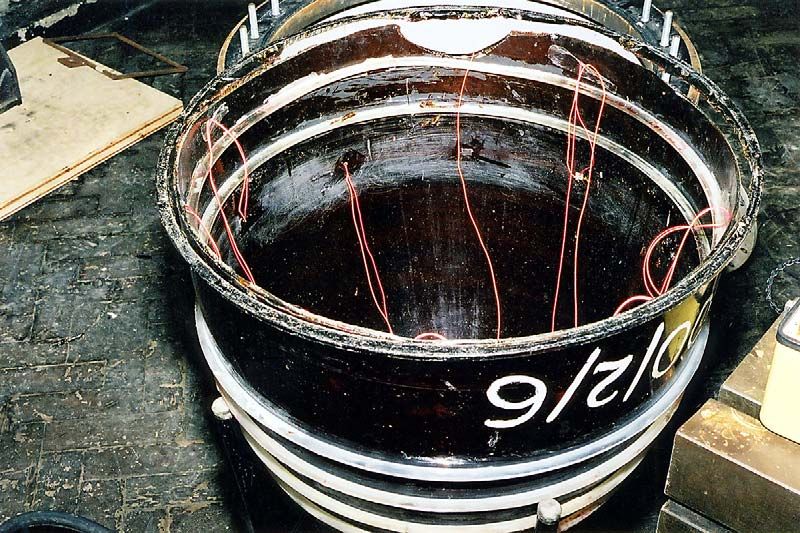
C.T.F. Ross et al. / Ocean Engineering 31 (2004) 1–19          3

  q       material density
  r1      principal longitudinal stresses
  r2      principal transverse stresses
  rx      in-plane meridional stress (of conical element)
  r/      in-plane circumferential stress (of conical element)
  s       in-plane shear stress
  s/x     in-plane shear stress (of conical element)
  t       Possion’s ratio
  qF      fluid density
  U       angle (azimuthal) around circumference of conical element
  v       flexural or twisting ‘‘strain’’
  x       angular (radian) frequency
  AR      aspect ratio
  SUP     solid urethane plastic

  Superscripts
  e       indicates an elemental property
  T       indicates the transpose of the matrix

that the pressure hull domes are usually slightly oblate, while the casing’s domes
are prolate and streamlined. The reason for this is that under external pressure, a
slightly oblate dome is stronger than a prolate dome.
   However, a slightly oblate dome is not hydrodynamically efficient and because of
this the casing’s forward dome is made streamlined and prolate; the result of which
necessitates the carrying of unwanted water in the forward end of the submarine.
   Now under external water pressure an oblate dome will buckle axisymmetrically
with its nose snapping through as shown in Fig. 2. In contrast, a prolate dome will
buckle in its flank through non-symmetric bifurcation buckling, as shown in Fig. 3.

                             Fig. 1. Submarine pressure hull.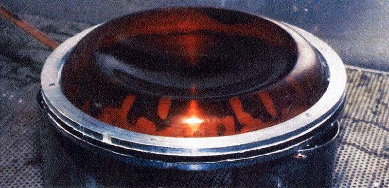
4                   C.T.F. Ross et al. / Ocean Engineering 31 (2004) 1–19

   Ross and Mackney (1983) found that prolate domes had poor resistance to the
effects of external pressure and to improve their structural characteristics, they sug-
gested ring stiffening the prolate dome in its flank, as shown in Fig. 4.
   The advantage of using a ring-stiffened prolate dome was that more space was
available in the submarine to carry whatever was necessary and less unwanted
water was transported. The idea of Ross and Mackney was used in the state-
of-the-art, but ill-fated submarine the Kursk (2000) and the highly successful
Trafalgar Class of submarines (2001). In the case of the latter, it appears that the
process allowed cruise missiles to be successfully launched through their forward
domes.
   Now one of the problems with military submarines is that they may vibrate and
transmit unwanted noises, which can be detected by the enemy; the modes of
vibration are shown in Fig. 5.
   From Fig. 5, it can be seen that these modes of vibration are of similar form to
the buckling modes shown in Fig. 3. Ross (1975) identified a dangerous type of
dynamic buckling mode. Ross argued that under increasing external pressure, the
compressive circumferential stresses would increase in magnitude, and this would
cause the pressure hull’s circumferential bending stiffness to decrease. The result of
this would be that the vessel’s resonant frequencies of vibration would also
decrease. According to Ross’ calculations, as the external pressure increased, not
only did the magnitudes of the resonant frequencies decrease, but the circumfer-
ential modes of vibration became of similar form to the circumferential buckling
modes. This prompted the alarming conclusion that if the buckling and vibration
modes of vibration were of similar form, there is a possibility that as a submarine
dived deeper into the water; the submarine pressure hull could collapse at a press-
ure considerably less than the static buckling pressure. It was not until 1987, some
years later that Ross et al. (1987a,b), Ross (2001) were able to prove this theory.
   In the present paper, the authors present a study, which is partly theoretical and
partly experimental, on the vibration of a large ring-stiffened prolate dome under
external water pressure; the dome is shown in Fig. 6.

2. Manufacture of the dome

  The dome, named AR 2.0, was made very accurately in a plastic called solid ure-
thane plastic (SUP). The dome was thermoset between accurately machined male
and female aluminium alloy moulds. The aspect ratio of the dome was nominally
2.0, where aspect ratio is defined as
                            Dome height
     Aspect ratio ðARÞ ¼
                            Base radius
The nominal radius of the dome was 0.25 m and its nominal wall thickness was
4 mm. Stiffening rings were attached to the dome as shown in Fig. 6.
   The first two ring stiffeners, near the base of the dome, were attached to the
internal surface of the dome wall to facilitate entry of the dome into the test tank.
C.T.F. Ross et al. / Ocean Engineering 31 (2004) 1–19 5
Fig. 2. Buckling of an oblate dome.
The other ring stiffeners were attached to the external surface of the dome, because
this process was easier than attaching them to the internal surface of the dome.
The material of construction of the rings was a polycarbonate and the adhesive
was a household epoxy resin, namely Araldite. The dome material had similar ten-
sile modulus and material densities. The spacing of the ring stiffeners was nomin-
Fig. 3. Buckling of a prolate dome.6 C.T.F. Ross et al. / Ocean Engineering 31 (2004) 1–19
Fig. 4. Ring-stiffened prolate domes.
ally 50 mm, starting from its base, and the number of ring stiffeners (N) attached
to the dome was 6.
The cross-section of each stiffener was shaped like a parallelogram of nominal
thickness 4 mm; as shown in Fig. 7.
Details of the ring stiffeners are seen in Table 1. The initial out-of-circularity of
the dome was found to be 0.75 mm.
To ensure that the ring stiffeners were firmly attached, fillets of Araldite adhesive
were added to the ring stiffener bases as shown in Fig. 8.
Fig. 5. Modes of vibration.C.T.F. Ross et al. / Ocean Engineering 31 (2004) 1–19 7
Fig. 6. Ring-stiffened prolate dome.
3. Experimental procedure
Test on the materials revealed the following:
SUP
Tensile modulus, E ¼ 2:9 GPa
Material density, q ¼ 1200 kg=m3
Poisson’s ratio, m ¼ 0:3 (assumed)
Tensile fracture stress, ryp ¼ 70 MPa
Fig. 7. Cross-section of a ring stiffener.8 C.T.F. Ross et al. / Ocean Engineering 31 (2004) 1–19
Table 1
Details of ring stiffeners (mm) of AR 2.0
Ring no D D1 D2 h (degrees)
1 493.1 465.5 465.92 3.04
2 485.09 457.05 457.91 6.18
3 470.35 469.68 471.02 9.50
4 450.9 449.99 451.83 13.11
5 437.72 422.48 424.96 17.21
6 388.06 386.44 389.68 22.09
Polycarbonate
E ¼ 2:6 GPa
q ¼ 1200 kg=m3
m ¼ 0:4
ryp ¼ 65:2 MPa
4. Assumptions
In the theoretical analysis E, q and m were assumed to be the same for all materi-
als and equal to the values found for SUP. The dome was first vibrated in air and
later under external water pressure, as shown in Fig. 9.
It can be seen from Fig. 9, that an excitation force was transmitted from an elec-
tromagnetic vibrator down to a rubber strap, so that the rubber strap excited the
flank of the dome through transverse tensile periodic forces in the rubber strap.
The rubber strap was stuck to the internal surface of the wall of the dome. The
rubber strap was pre-tensioned across the diameter of the dome. The excitation
force from the vibrator was transmitted to the rubber strap via a slim vertical
metal rod. The rubber strap was also firmly attached to the slim vertical rod.
Fig. 8. Ring stiffeners with Araldite fillets.C.T.F. Ross et al. / Ocean Engineering 31 (2004) 1–19 9
Fig. 9. Dome vibration apparatus.
5. Experimental procedure
The electrical circuit is shown schematically in Fig. 10. The dome was vibrated
both in air (a) and then while submerged in water (b).
5.1. Vibration in air
Fig. 10 shows the way the data was processed and recorded during the experi-
ment. The signal generator was used to set the different frequencies for vibration.
The response of the various vibrations was measured with an accelerometer con-
nected to an oscilloscope. The oscilloscope was set to display two sine waves, one
representing the output from the signal generator and the other representing the
output from the accelerometer.
The vibrator generating the oscillation was attached via a rod to a rubber strap
fixed on the inside of the dome, shown in Fig. 9.
In order to find the different natural frequencies in air, that the dome would be
likely to vibrate in (i.e. n ¼ 2, n ¼ 3, n ¼ 4), only one half of the dome (180 degrees
circumferentially) needed investigation. By adjusting the signal generator, a range
of frequencies could be scanned through. The amplitude of the sine wave generated
Fig. 10. Electrical circuit for the vibration analysis.10 C.T.F. Ross et al. / Ocean Engineering 31 (2004) 1–19 by the signal generator was displayed on the oscilloscope and varied accordingly. The accelerometer was attached to the inside surface of the dome with the aid of a small piece of wax. When the dome was first excited, the accelerometer was moved around the internal surface of the dome until a maximum amplitude was detected. When the maximum amplitude was detected, it was then necessary to find out which eigenmode this frequency corresponded to. The accelerometer was then placed just above the points where the rubber strap had been attached to the internal wall of the dome. The accelerometer was then moved circumferentially around the inside of the dome and readings were taken at increments of 10 degrees, right up to the other end of the rubber strap, thus cover- ing 180 degrees in total. This was done to observe the circumferential mode shape of vibration. Having found the natural frequencies of vibration, the nodes and anti-nodes could easily be determined; these described the modal pattern of vibration for n ¼ 2, n ¼ 3, n ¼ 4. The experimentally determined frequencies of vibration in air are shown in Table 2. A typical plot of the variation of phase angle with the azimuthal angle is shown in Fig. 11. The figure shows the nodes and anti-nodes as both positive, hence, for n ¼ 3, there were six peaks and for n ¼ 4, there were eight peaks. 5.2. Vibration in water The vessel was submerged in water as can be seen in Fig. 9. Having opened the overflow of the tank shown in Fig. 9, the system was bled to ensure that no air was trapped. Initially the pressure was at zero bar. The resonant frequencies in water were expected to lie below the natural frequencies previously found in air. The experimental procedure for finding the resonant frequencies in water was no differ- ent to the experimental procedure in air. However, when the natural frequencies in water for n ¼ 2, n ¼ 3, n ¼ 4 were found, different values of external pressure were applied for different values of n. In each case, a drop in frequency became apparent as the external hydrostatic press- ure was increased; this resulted in the amplitude of the sine wave of the signal gen- erator becoming smaller. The frequencies were then re-adjusted on the amplifier, until the output waves reached their maximum amplitude again (Table 3). Typical variations of phase angle with the azimuthal angle for AR 2.0 in water, is shown in Fig. 12. Table 2 Experimentally determined natural frequencies in air (Hz) n 1 2 3 4 Frequency 270 350 420 480
C.T.F. Ross et al. / Ocean Engineering 31 (2004) 1–19          11

                              Fig. 11. Variation of the phase angle for AR2.0.

6. Theoretical analysis

  The theoretical analysis was via the finite element method, where a pair of cou-
pled matrix equations were merged together and then solved. One equation was
used to represent the vibration of the structure, namely Eq. (1), and the other
equation was used to represent the motion of the fluid, namely Eq. (2). Details of
these equations are given in Ross (2001) and Zienkiewicz and Newton (1969).
                           @fui g       @ 2 fui g    1
       ½Kfui g þ ½Cv            þ ½M      2
                                                  þ    ½ST fPi g þ fRg ¼ 0              ð1Þ
                            @t            @t        qF
where,

                      @2             @ 2 fUi g
        ½HfPi g þ ½G 2 fPi g þ ½S           ¼0                                        ð2Þ
              P e @t                    @t2
        ½H ¼ ½h

Table 3
Experimental resonant frequencies for AR 2.0 in water (Hz)
Pressure (Ib f/in.2)   Pressure (bar)      n¼2                  n¼3                n¼4
0                      0                   84                   105                140
10                     0.69                80                   103                136
20                     1.38                76                   101                130
25                     1.72                75                   100                128
30                     2.07                72                    99                124
12 C.T.F. Ross et al. / Ocean Engineering 31 (2004) 1–19
Fig. 12. Vibration of phase angle for AR 2.0 at 105 Hz (n ¼ 3).
ð
@½NT @½N @½NT @½N @½NT @½N
for ½he ¼ þ þ dx dy dz
ve @x @x @y @y @z @z
and
X ð
1
½G ¼ P ½ge for ½ge ¼ ½NT ½Ndx dy dz
½S ¼ ½s e c2 ve
ð
½se ¼ qF ½NT ½Nds
ge
For free vibrations without damping, Eq. (1) reduces to
@ 2 fUi g 1 T
½KfUi g þ ½M þ ½S fPi g ¼ f0g ð3Þ
@t2 qF
Under external pressure Eq. (3) becomes
@ 2 fUi g 1 T
½K fUi g þ ½M 2
þ ½S fPi g ¼ f0g ð4Þ
@t qF
where
½K ¼ ½K þ ½KG
.
If the fluid–structure vibrates with simple harmonic motion, it is reasonable to
assume that the vector of nodal acoustic pressures {Pi} and the vector of nodal dis-C.T.F. Ross et al. / Ocean Engineering 31 (2004) 1–19 13
placements {Ui} are given by
fPi g ¼ fP0 gcosxt
and
fUi g ¼ fu0 gcosxt
Coupling Eqs. (2) and (4) leads to the following sets of simultaneous equations:
½K ½ST =qF u0 2 ½M 0 u0
x ¼0 ð5Þ
0 ½M P0 ½S ½G P0
The solution of Eq. (5) is computationally inefficient, because of its unsymmetrical
form. However, Irons (1965) has shown that this equation can be written in the
following symmetrical form:
" #
qF ½K 0 u0 T 1 T
2 qF ½M þ ½S ½H ½S ½S ½H ½G
1
x
0 ½G P0 ½G½H 1 ½S ½G½H 1 ½G
u0
¼0 ð6Þ
P0
where½ST ½H 1 ½SZ is termed the added mass matrix. Solution of Eq. (6) can be
carried out using standard eigenvalue techniques, including the simultaneous iter-
ation method of Jennings (1977).
The theoretical analysis of the vibration of pressure vessels has been carried out
using a finite element program (VIBCONER), which is outlined in Ross (1984).
The program uses a truncated conical axisymmetric element with two nodal circles;
each node has four degrees of freedom (i.e. eight per element). The axisymmetric
element used for modelling the structure is shown in Fig. 13. The program deter-
mines the eigenmodes by superimposing deformations for each vibration mode. A
reduction process due to Irons (1970) has enabled the size of the stiffness matrix to
be reduced by a factor of about four, thus providing a very efficient program in
terms of computer memory, and indeed speed.
The truncated conical shell element which was used by Ross (1974) is shown in
Fig. 13, where it can be seen that the element was described, by nodal circles at its
ends.
Ross (1974) assumed the following displacement functions for the three displace-
ments u, v and w:
u ¼ ½ui ð1 fÞ þ uj fcosn/
v ¼ ½vi ð1 fÞ þ vj fsinn/
ð7Þ
w ¼ ½ð1 3f2 þ 2f3 Þwi þ lðf 2f2 þ f3 Þhi þ ð3f2 2f3 Þwj
þlð f2 þ f3 Þhj cosn/
fUg ¼ ½NfUi g ð8Þ
The assumed displacement functions for {U} allowed for a sinusoidal distri-
bution in the circumferential direction to cater for the lobes of Fig. 2.14 C.T.F. Ross et al. / Ocean Engineering 31 (2004) 1–19
The stiffness matrix was given by
ð1
½k ¼ lp½DC r½B1 T ½D½B1 df½DC; ð9Þ
0
where
r ¼ Ri þ ðRj Ri Þf
ð10Þ
½B ¼ ½B1 ðeither cosn/ or sinn/Þ
and
feg ¼ ½BfUi g ð11Þ
8 9
>
> ex >
>
>
> e/ >
>
>
> >
>
> vx > >
>
> >
>
> v > >
: / > ;
8 v x/ 9
>
> ux >
>
>
> ð1=rÞv/ þ ð1=rÞðusina wcosaÞ >
>
>
> >
>
< ð1=rÞu þ v ð1=rÞðvsinaÞ =
/ x
¼
>
> wxx >
>
>
> 2 >
>
>
> ð1=r Þw// þ ð1=r2 Þv/ cosa þ ðsina=rÞwx >
>
: ;
2 ð1=rÞwx/ ð1=r2 Þw/ sina þ ð1=rÞvx cosa ð1=r2 Þvsinacosa
ð12Þ
The relationship between local and global displacements was
fUi g ¼ ½DC Ui0 ¼ ½ ui vi wi hi uj vj wj hj ð13Þ
where
2 3
c 0 s 0
6 0 1 0 0 7
6 04 7
6 s 0 c 0 7
6 7
6 0 0 0 1 7
½DC ¼ 6 ð14Þ
6 c 0 s 077
6 7
6 0 1 0 07
4 04 5
s 0 c 0
0 0 0 1C.T.F. Ross et al. / Ocean Engineering 31 (2004) 1–19 15
The geometrical stiffness matrix [KG] was obtained from the matrix of strains
due to large displacements (2000), as follows:
8 2 9
8 9 >
> wx >
>
>
>
< dex = 1 > < v w/ 2 > =
feL g ¼ de/ ¼ þ ð15Þ
: ; 2> r r >
dex/ >
> wx w/ >
>
>
:2 >
;
r
As the normal stresses rx and r/ in the x and / directions, respectively, are princi-
pal stresses, the shear stress in the x–/ plane is zero, hence Eq. (15) simplifies to:
" #( )
1 wx 0 wx
feL g ¼ ðv þ w/ Þ ðv þ w/ Þ ð16Þ
2 0
r r
Using the same notation as Zienkiewicz and Taylor (2000)
( )
wx
ðv þ w/ Þ ¼ ½GfUg ð17Þ
r
The geometrical stiffness matrix was then obtained from [k1], where ½G ¼
½G1 ðeither cos n/ or sin n/Þ
ð
½k1 ¼ ½DCT ½GT ½r½GdðvolÞ½DC
ð vol
¼ ½DCT ½GT ½r½Grd/dxdz½DC
volð
1
¼ ½DCT plt r½G 1 T ½r½G 1 df½DC
ð 01
T 1 T rx 0
¼ ½DC plt r½G ½G 1 df½DC ð18Þ
0 0 r/
and
pr
rx ¼
2tcosa
pr
r/ ¼ cosa ð19Þ
t
The element mass matrix was given by
ð1
½m0 ¼ ½DCT ½NT q½Ntr d/l df½DC ð20Þ
016 C.T.F. Ross et al. / Ocean Engineering 31 (2004) 1–19
Table 4
Theoretical frequencies for AR 2.0 (Hz)
Pressure (bar) n¼1 n¼2 n¼3 n¼4
0 89 117 126 141
0.69 89 115 123 135
1.38 88 114 119 128
1.72 88 114 118 124
2.07 88 113 116 120
where
½N ¼ ½N 1 ðeither cosn/ or sinn/Þ ð21Þ
ð1
½m ¼ ½DC qtlp r½N 1 T ½N 1 df½DC;
0 T
0
where
r ¼ Ri þ ðRj Rj Þf
The integrations were carried out numerically, using four Gauss points in the f
direction.
The element used to represent the fluid motion was a solid annular element,
which had a cross-section of an eight-node isoparametric form and 1 degree of
freedom per mode, namely P. The program used was called SUBPRESS; it was for
isotropic materials. It used axisymmetric structural elements and axisymmetric
fluid elements.
7. Results
The theoretical results, for the vibrating under external water pressure for the
dome is shown in Table 4.
Fig. 13. Truncated conical shell elements used for modelling the structure.C.T.F. Ross et al. / Ocean Engineering 31 (2004) 1–19 17 Fig. 14. Comparison between theoretical and experimental resonant frequencies for AR 2.0 at zero pressure. Comparisons between theory and experiment for AR 2.0 are shown in Figs. 14–17. The theoretical buckling pressure for the dome was found to be : 4.41 bar. Although the resonant frequencies decreased with increasing external pressure, as the applied external pressures were only 0.47 of Pcr for AR 2.0, the fall in the magnitudes of the resonant frequencies was not large. These experimentally applied pressures were deliberately kept low to avoid acci- dentally buckling the dome during vibration. It can be seen that the theoretical and experimental resonant frequencies decrease in magnitude with increasing external water pressure and that there is good correlation between the two. Fig. 15. Comparison between theoretical and experimental resonant frequencies for AR 2.0 at various pressures (n ¼ 2).
18                      C.T.F. Ross et al. / Ocean Engineering 31 (2004) 1–19

Fig. 16. Comparison between theoretical and experimental resonant frequencies for AR 2.0 at various
pressures (n ¼ 3).

Fig. 17. Comparison between the theoretical and experimental resonant frequencies for AR 2.0 at vari-
ous pressures (n ¼ 4).

8. Conclusions

  The effect of ring-stiffening the flank of the dome was to considerably increase
the stiffness of the dome and its resonant frequencies. The effect was more pro-
nounced in water than in air. The effect of water was to decrease the resonant fre-
quencies of the domes in air by a factor of about 3 in many cases.
  The theoretical and the experimental results showed good agreement and also
that as the externally applied pressures were increased, the resonant frequencies
decreased. This effect was not large in the investigation conducted, because the
experimentally applied water pressures during vibration were only about from 0.25
to 0.33 of the theoretical buckling pressures of the domes.

References
Anon., 2000. Inside the Kursk, Daily Mail, 7, August 15.
Anon., 2001. Inside HMS Triumph, Daily Mail, 7, October 1.
C.T.F. Ross et al. / Ocean Engineering 31 (2004) 1–19                        19

Ross, C.T.F., 1974. Lobar buckling of thin-walled cylindrical and truncated conical shells under external
   pressure. S.N.A.M.E., J. Ship. Res. 18, 272–277.
Ross, C.T.F., 1975. Finite elements for the vibration of cones and cylinders. IJNME 9, 833–845.
Ross, C.T.F., 1984. Finite Element Programs for Axisymmetric Problems in Engineering. Horwood,
   Chichester, UK.
Ross, C.T.F., 2001. Pressure Vessels: External Pressure Technology. Horwood Publishing Ltd, Chiche-
   ster, UK.
Ross, C.T.F., Emile, Johns, T., 1987a. Vibration of thin walled domes under external water pressure. J.
   Sound Vib. 114, 453–463.
Ross, C.T.F., Johns, T., Emile, 1987b. Dynamic buckling of thin walled domes under external pressure.
   In: Tooth, A.S., Spence, J. (Eds.), Applied Solid Mechanics. second ed. Elsevier Applied Science,
   pp. 211–224.
Ross, C.T.F., Mackney, M.D.A., 1983. Deformation and stability studies of thin-walled domes under
   uniform pressure. I. Mech. E., J. Strain Anal. 18, 167–172.
Irons, B., 1965. Structural eigenvalue problems: elimination of unwanted variables. JAIAA 3, 961.
Irons, B.M., 1970. Role of part-inversion in fluid–structure problems with mixed variables. JAIAA 7,
   568.
Jennings, A., 1977. Matrix Computation for Engineers and Scientists. Wiley, Chichester, UK.
Zienkiewicz, O.C., Newton, R.E., 1969. Coupled vibrations of a structure submerged in a compressible
   fluid. In: International Symposium on Finite Element Techniques, University of Stuttgart, Germany.
Zienkiewicz, O.C., Taylor, R.L., 2000. The Finite Element Method. fifth ed. Butterworth-Heinemann,
   Oxford, UK, (vols. 1, 2 & 3).
You can also read