Research on Wasp population based on Gray Prediction and Fuzzy Analytic hierarchy process

Journal of Physics: Conference Series

PAPER • OPEN ACCESS

Research on Wasp population based on Gray Prediction and Fuzzy
Analytic hierarchy process
To cite this article: Xinyuan Wu et al 2021 J. Phys.: Conf. Ser. 1952 042071

View the article online for updates and enhancements.

 This content was downloaded from IP address 46.4.80.155 on 01/10/2021 at 01:43

IPEC 2021 IOP Publishing
Journal of Physics: Conference Series 1952 (2021) 042071 doi:10.1088/1742-6596/1952/4/042071

Research on Wasp population based on Gray Prediction and
Fuzzy Analytic hierarchy process

 Xinyuan Wu1, *, Yujia Wu1, Xiaohan Xu2
 1
 Jinan University-University of Birmingham Joint Institute of Jinan University,
 Guangzhou, 511486, China
 2
 Institute for Economic and Social Research of Jinan University, Guangzhou, 511486,
 China

 *Corresponding author: xinyuanwu1998@jnu.edu.cn

 Abstract. The invasion of exotic species should be paid attention to because of its severe
 consequences, and governments have constructed monitoring and tracking system to
 collect people’s sightings of species. For example, Asian giant hornet, an exotic species
 for North American countries was first discovered in September, 2019. Interpretations
 based on received reports are of essential to master the current situation of species and
 to predict its spread. However, there is a considerable number of mistake reports, it is
 necessary to select the most likely positive reports out of mountains of reports to be
 detailly investigate first. In this paper, two main problems are focused: interpretation of
 historical reports and strategy of prioritization. First of all, this paper preprocesses the
 image data based on Gaussian filtering and convolution neural network to make it as
 balanced as possible. In addition, the image consists of a wide range of array data.
 Proper treatment can improve the efficiency of analysis. Then, construct the GPSM
 model (Gray Predicting Spread Model) based on gray prediction to measure the spread
 of the pest. From the historical positive sighting location provided in the dataset, the
 GPSM model is able to output the predicted next location following the previous
 principle. If the distance between predicted location and current outbreak area are
 significant, a spread can be concluded. Tests for the GPSM model shows the model has
 a very high level of precision

 Keywords: Hornet, image recognition system, the GPSM model, the Prioritizing
 Judgment model.

1. Introduction
The invasion of exotic species is getting more and more attention in the last few decades since it can
change and even damage the local biodiversity and ecosystem [1]. Since the difference of living habit
and absence of natural enemy in local ecosystem, exotic species can reproduce without limit and occupy
the limited resources, leading local species to die. Therefore, government has created helplines and
websites for people to report their sightings. It is essential using these reports to detect the existence and
current situation of exotic species and predict their spread [2].

 Content from this work may be used under the terms of the Creative Commons Attribution 3.0 licence. Any further distribution
 of this work must maintain attribution to the author(s) and the title of the work, journal citation and DOI.
Published under licence by IOP Publishing Ltd 1

IPEC 2021 IOP Publishing
Journal of Physics: Conference Series 1952 (2021) 042071 doi:10.1088/1742-6596/1952/4/042071

 This article verifies all reports and produces complete data sets, classifying each report as positive
or negative. Then explain the reports received, determine whether the spread of pests can be predicted,
and give the level of accuracy of the prediction.

2. Data preprocessing based on convolution Neural Network

2.1. Convolution neural network
 Step 1: Defining training set and test set
 Given the image data after processing, the data will be randomly split into two set based on the lab
status that respectively contain 80% and 20% of the raw data. The bigger data will be used to train our
CNN model and the other one will be used to test the accuracy of the identification. Here the classes
will be the lab status.
 Step 2: Constructing convolutional layers
 At each convolutional layer, the dataset will be packed into an input cube that is convoluted with
multiple feature maps. For our image data ,it will be enclosed into a matrix of ,where
 refers to the spatial size of the data, is the number of the channels and is the -th feature map
of the matrix. Define there will be filters at this convolutional layer and the -th filter can be
characterized by the weight and bias .The -th output can be generate through this formula:

 ∑ ∙ (1)

 Where 1,2, ⋯ , , ∙ represents the convolution operator and is the function to improve the
nonlinearity of the network.
 Step 3: Constructing pooling layers
 The layers are created to reduce the size of feature maps in the previous layers to obtain more general
and abstract features within classes. Due to the existence of the redundant information, the pooling layers
are periodically inserted after several convolutional layers. Reducing the spatial size of the feature maps
progressively, the pooling layers will decrease the number of parameters and computation of the network.
For the window-size neighbor ,the average pooling operation will be:

 ∑ , ∈ (2)

 where is the number of the elements in the neighbor and is the activation value at , .
 Step 4: Constructing a fully connected layer
 At the last step of the network construction, the feature maps of the previous layers are flattened and
fed to this layer. The fully connected layers will be:

 ∑ (3)

 Where , , and are the input data, output label, weight and bias of the fully connected layers.

 2

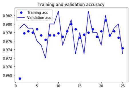
IPEC 2021 IOP Publishing
Journal of Physics: Conference Series 1952 (2021) 042071 doi:10.1088/1742-6596/1952/4/042071

2.2. Results

 Figure 1. Accuracy of results

 Due to the data limitation, the accuracy seems not to be significantly improved a lot and stays at
around 0.98 when more learning is done. However, through the progress of multi-layers learning of the
training set, the validation loss has a downward trend which implies that the CNN model will be more
efficient when more data is reported.

3. The GPSM Model
In this section, the paper proposes the GPSM model (Gray Predicting Spread Model) to predict the
spread of the Asian giant hornet can be predicted [3] [4]. The main process of our model is to operate
gray prediction based on gray model. The GPSM model is constructed based on the idea of gray
prediction. The gray system is an unascertained information system containing both the known and
unknown information. This property makes the GPSM model outputting accurate predictions.

3.1. Model Overview
The purpose of this model is to predict the sighting location of next time unit. Specific process shown
below is to predict the latitude of the location, and its longitude can be obtained by operating the same
method [5].
 By approximately analyze the dataset given and the background information of the occurrence of
Asian giant hornet, a month is the appropriate time unit. Take the average latitude and longitude of a
month to be the average sighting location of the month [6]. If the distance between the predicted location
and the average current sighting location is larger than the critical value, then the spread of Asian giant
hornet can be concluded.

3.2. Steps of GPSM Model
From the dataset given, the positive reports are all clustered in the same area, and the attached file shows
the Asian giant hornet is found in September 2019, which is not far from today. Hence, take every month
to be a time unit. The dataset provided gives 14 positive reports in total from September 2019 to October
2020.
 Step 1: Data examining and adjusting
 From the dataset given, calculate the average latitude of the sighting spot, expressed it as:

 1 , 2 ,⋯, (4)

 To guarantee the effectiveness of gray prediction, step ratio of the sequence should be checked. Step
ratio is calculated by:

 3

IPEC 2021 IOP Publishing
Journal of Physics: Conference Series 1952 (2021) 042071 doi:10.1088/1742-6596/1952/4/042071

 (5)

 If all step ratio are in the range , , then sequence can be used as model
GM (1, 1) and implement gray prediction. Otherwise, sequence should be switched to fall in the
range, and an appropriate constant is needed to translate:

 1,2, ⋯ , (6)

 to make sequence 1 , 2 ,⋯, has step ratio

 ∈ 2,3, ⋯ , (7)

 Step 2: Construct model GM (1,1)
 Operate the accumulated generating process on the original sequence to obtain a new sequence:

 1 , 2 ,⋯, (8)

 Where ∑ . Define the gray derivative of to be:

 1 (9)

 is the one-time accumulated generating sequence, and in the gray prediction model, is
sufficient to predict and it’s not essential to accumulate more times.
 Define to be the mean sequence of :

 0.5 0.5 1 (10)

 and 2 , 3 ,⋯ .
 Then, the gray differential equation model of GM (1,1) is defined to be:

 (11)

 i.e.

 (12)

 In this equation, is called gray derivative, developing derivative, whitening
background value, and graying quantity.

 Its corresponding whitening differential equation is:

 (13)

 4

IPEC 2021 IOP Publishing
Journal of Physics: Conference Series 1952 (2021) 042071 doi:10.1088/1742-6596/1952/4/042071

 2 1
 ⎡ ⎤
 Define , , 2 , 3 ,⋯ , ⎢ 3 1⎥.
 ⎢ ⋮ ⋮⎥
 ⎣ 1⎦
 Here gives the method to determine vector , if ∙ exists, then by least square method,

 , ∙ 
 (14)

 Therefore, by solving the whitening differential equation, it can be obtained that:

 1 1 1,2, ⋯ , 1 (15)

 And 1 1 1,2, ⋯ , 1 .
 Step 3: Test predicting value
 Since the future value is unknown, this paper use step ratio deviation value to test precision. Calculate
step ratio by 1 and , then combine to obtain corresponding step ratio
deviation:

 .
 1 (16)
 .

 If 0.2 , then the prediction meets the normal standard, and if 0.1 , then the
prediction meets a high standard.

3.3. Results of GPSM Model
The model gives the developing derivative 2.0035 10 , graying quantity 122.7698.
Similarly, in the process of predicting longitude, the developing derivative 1.2767 10 ,
graying quantity 48.9885 . Then, with these estimations, their corresponding whitening
differential equations can be obtained.
 The predicted latitude and longitude are obtained and the outcomes are shown as Figure 2:

 Figure 2. Predicted location
 predicted latitude: 48.9291; predicted longitude: -122.5362

 5

IPEC 2021 IOP Publishing
Journal of Physics: Conference Series 1952 (2021) 042071 doi:10.1088/1742-6596/1952/4/042071

 Figure 2 indicates that for most months, the predicted locations are precise while there is a significant
difference in June. Our GPSM model gives the predicted next location having latitude 48.9291 and
longitude 122.5362. From the past data, predict a location of Asian giant hornet in June which has a
significant difference to its actual location. Therefore, it can be deduced that a spread might exists in
June.
 The level of precision of the GPSM model is indicated by the step ratio deviation. The step ratio
deviation of latitude and longitude predictions are:

 Table 1. Step ratio deviation of predicted location
 month/month 1/2 2/3 3/4 4/5
 latitude -0.0019 0.0012 -0.0008 0.0007
 longitude -0.0049 0.0011 -0.0008 -0.0001
 month/month 5/6 6/7 7/8 8/9
 latitude -0.0046 0.0032 0.0013 0.0001
 longitude -0.0017 0.0029 -0.0012 0.0002

 It can be seen that all step ratio deviations are under 0.2, which means our prediction meets a high
standard of precision.

4. The Prioritizing Judgment Model
The paper designs the Prioritizing Judgment Model to evaluate key factors deciding the likelihood of
correct classification and capture information of reports to provide a strategy of prioritizing.

4.1. Determining the weight for each factor
 (A) Season-A1: According to the background information of Pennsylvania State University, Asian
bumblebee is one-year biological species. There are obvious differences in the number of populations
in different seasons. Therefore, the season is a factor to be considered.
 (B) Location-A2: Asian bumblebee mainly occurs in specific areas, with little change in latitude and
longitude. At the same time, the paper should be on guard against the possible spread and movement of
pests. Therefore, the location is a factor determining positive sightings, while the distance from the
outbreak area and the number of recent reports in the area are detailed factors in determining whether
the site is important or not.
 (C) Image recognition-A3: Despite the picture itself and the content of notes, the form of report is
also a meaningful information contributing to the likelihood of positive classification. Report with more
pictures and concrete note are preferred.

4.2. 3.2 Fuzzy Preferential Relation Matrix
In fuzzy analytic hierarchy process, preferential relation matrix is a matrix with three possible elements
 0,0.5,1 . The meaning of preferential relation matrix is:

 Table 2. Value of elements in preferential relation matrix
 Degree of importance
 1 is more important than 
 0.5 and have the same importance
 0 is less important than 

 For the level indicators and secondary indicators listed in the prioritizing judging system, their
preferential relation matrix should be confirmed. Denote the preferential relation matrix of level

 6

IPEC 2021 IOP Publishing
Journal of Physics: Conference Series 1952 (2021) 042071 doi:10.1088/1742-6596/1952/4/042071

indicators to be , the degree of membership in is obtained by summing up 
according to rows, i.e. ∑ .

 Table 3. Relation matrix of level indicators-A
 A1 A2 A3 
 A1 0.5 0 0 0.5
 A2 1 0.5 0 1.5
 A3 1 1 0.5 2.5

 The prioritizing relation is .
 Applying the same method, the preferential relation matrix of two secondary indicators under A1
(season), denoted by is given by:

 Table 4. Relation matrix of level indicators-A1
 B11 B12 
 B11 0.5 0 0.5
 B12 1 0.5 1.5

 As an annual species building nests every year the current nests will be abandoned and the only
individuals surviving are fertilized queens at winters. During spring and summer next year, the growth
of Asian giant hornets is slow and its population reaches peak around August. After male and queens
are produced and begin to leave, the colony falls to disarray and finally die out in winter. By its life
history, the prioritizing relation is & & .
 Following the same method, the preferential relation matrix of two secondary indicators under A2
(location), denoted by is given by:

 Table 5. Relation matrix of level indicators-A2
 B21 B22 
 B21 0.5 1 1.5
 B22 0 0.5 0.5

 The prioritizing relation is . We believe
locations near the outbreak area are more likely to sight the pest.

4.3. Weight of indicator
With formulas ℎ 0.5 and ∑
 , in which ℎ ∏ ℎ . ℎ is the element of
the -th row and -th column, is the weight of the -th indicator.
 By calculation, the weight for each level indicator is shown as matrix . The weight for image
recognition 0.4543 is larger than the weight for location 0.3348 , which is larger than the weight
for season 0.2109 .

 7

IPEC 2021 IOP Publishing
Journal of Physics: Conference Series 1952 (2021) 042071 doi:10.1088/1742-6596/1952/4/042071

 Table 6. Index weight matrix-A
 A1 A2 A3 
 A1 0.5 0.333 0.167 0.2109
 A2 0.667 0.5 0.333 0.3348
 A3 0.833 0.667 0.5 0.4543

 The weight for secondary indicators under A1 (season) is shown as matrix . Weights for two
indicators are & 0.634 and & 0.634 :

 Table 7. Index weight matrix-A1
 B11 B12 
 B11 0.5 0.25 0.366
 B12 0.75 0.5 0.634

 Similarly, the weight for secondary indicator under A2 (location) is shown as matrix . Weights
for two indicators are 0.634 , and 0.366 :

 Table 8. Index weight matrix-A2
 B21 B22 Wi
 B21 0.5 0.75 0.634
 B22 0.25 0.5 0.366

4.4. Results
 (1) Mark for A1(season)
 To avoid falling into dummy variable trap, we combine the mark and weight for secondary indicators.
If the report has a season that is winter & spring, it is marked 0.366. Otherwise, it is marked 0.634.

 Figure 3. Periodicity

 (2) Mark for A2(location)
 From the living habit of Asian giant hornet, a new queen has a range of 30km for building her new
nest. Hence, it is possible to sight the pest in 30km around. On the basis of the outbreak area drawn,
enlarge the radius by 30km to obtain circle A, then continuously enlarge the radius of circle A by 30km
and obtain circle B.

 8

IPEC 2021 IOP Publishing
Journal of Physics: Conference Series 1952 (2021) 042071 doi:10.1088/1742-6596/1952/4/042071

 Figure 4. Distance towards outbreak area

 Table 9. Marks for different regions
 Outbreak area 1
 2
 Circle A
 3
 1
 Circle B
 3
 (3) Mark for A2(image recognition)
 By continuously adding in more image into the model, the level of precision increase with a longer
training time. However, it is never impossible for the model to have a precision of 100%, and outcomes
of this algorithm can only be part of the judgment evidence.
 It is believed that reports with image recognition outcome “positive” is more likely to be a positive
sighting than those with outcome “negative”. Reports with outcome “positive” is marked 0.7, while
reports with outcome “negative” is marked 0.3.

5. Conclusion
The invasion of alien species has serious consequences, which should be paid great attention to. This
paper mainly focuses on historical data and optimization strategies to study the population invasion
behavior of alien species-Asian wasp. First of all, the convolution neural network is used for data
processing, and then the gray prediction of the image array is carried out to get the data of the next
location. Then combined with the fuzzy analytic hierarchy process, quantify the season, location, image
recognition three indicators to determine the event. Appropriate choice of data processing method.
According to the main idea of Gaussian filter and convolutional neural network, our image recognition
system enlarges sample size, balances ratio of different samples, improves predicting precision and
increases calculating speed.

References
[1] Shutao Li, Weiwei Song, Leyuan Fang, Yushi Chen, Pedram Ghamisi, J´on Atli Benediktsson.
 Deep Learning for Hyperspectral Image Classification: An Overview [J]. IEEE.
[2] Studies on Applying Gray System Theory to Forecasting Population Dynamic of Rodent [J].
 Journal of August 1st Agri. College, 1992 (01): 63 - 68.
[3] Cai MuZhen,Dong Bo,Xiao Yuhui. Prediction of Fish School based on Neural Network and Gray
 Prediction[J]. Journal of Physics: Conference Series, 2021, 1802 (4).
[4] Qihong Zhou,Guangzong Wu, Zhenxi Wang,Bing Wang, Ge Chen, Zhihong Sun. Analysis and
 prediction of the width of spreading carbon fiber tow based on gray system theory [J]. Journal
 of Applied Polymer Science, 2021, 138 (12).
[5] Wang Shu, Li Hao, Zhong Ke, Nie Shan, Zhou Wenan. Application of fractional prediction model
 based on improved grayscale algorithm [J]. Electronic Technology and Software Engineering,

 9

IPEC 2021 IOP Publishing
Journal of Physics: Conference Series 1952 (2021) 042071 doi:10.1088/1742-6596/1952/4/042071

 2020 (11): 212 - 215.
[6] Shan Zhilong, Liu Lanhui, Zhang Yingsheng, Huang Guangxiong. A strong adaptive mobile node
 location algorithm using grayscale prediction model [J]. Journal of Electronics and
 Information, 2014 1492 36 (06): 2014 - 1497.

 10