How to Win the House: NBA Odds Analysis and Predictions - Scientific Research ...
←
→
Page content transcription
If your browser does not render page correctly, please read the page content below
Open Journal of Social Sciences, 2021, 9, 177-187
                                                                                                  https://www.scirp.org/journal/jss
                                                                                                             ISSN Online: 2327-5960
                                                                                                               ISSN Print: 2327-5952

How to Win the House: NBA Odds Analysis and
Predictions

Wenpeng Di1, Bin Yuan2, Haiyi Wen3
1
  College of Letters & Science, UC Santa Barbara, Santa Barbara, CA, USA
2
  School of Traffic and Transportation, Chongqing Jiaotong University, Chongqing, China
3
  Wuhan Britain-China School, Wuhan, China

How to cite this paper: Di, W. P., Yuan, B.,     Abstract
& Wen, H. Y. (2021). How to Win the House:
NBA Odds Analysis and Predictions. Open          In recent years, odd-making systems, from automated bookmakers and com-
Journal of Social Sciences, 9, 177-187.          puter casino software to sophisticated market-research tools for betting and
https://doi.org/10.4236/jss.2021.92013
                                                 investment, have increasingly sought to capture the most accurate spread of
Received: December 11, 2020
                                                 outcome probabilities, and so betting odds have been increasingly dominated
Accepted: February 16, 2021                      by algorithms for generating the spread (Spann & Skiera, 2009). This study
Published: February 19, 2021                     analyzes NBA betting spreads and odds in the 2016-2017 season to investigate
                                                 the degree to which these odds have succeeded in capturing the spread of the
Copyright © 2021 by author(s) and
Scientific Research Publishing Inc.
                                                 game in real-life. In this paper, models are developed by the method of mul-
This work is licensed under the Creative         tiple linear regression to predict the results of the game based on the team’s
Commons Attribution International                past performance. The model can help bookmakers optimize their algorithms.
License (CC BY 4.0).
                                                 By reading this paper can also help the normal players with weak statistical
http://creativecommons.org/licenses/by/4.0/
                                                 base understand how the game works.
                Open Access

                                                 Keywords
                                                 NBA Ranking, Linear Regressions, Dummy Variable

                                               1. Introduction
                                               Sports betting has exploded over the last few years (Humphreys, Paul, & Wein-
                                               bach, 2013), with the total market value of this complex enterprise peaking at
                                               over $85 billion in 2019 and projected to exceed $100 billion by 2022. However,
                                               the most challenging aspect about betting is the perennial question: how do bet-
                                               tors win against the house? Bettors look at spreadsheets, forms of the
                                               teams/players, and other types of information to predict the outcome of the
                                               game but are left with the dilemma of how to best make a rational decision on
                                               which strategy to employ and to the extent to which each is best supported by

DOI: 10.4236/jss.2021.92013        Feb. 19, 2021                   177                              Open Journal of Social Sciences
W. P. Di et al.
information available to maximize their chances of winning (Golec & Tamarkin ,
1995).
The purpose of this paper is to identify a possible research model for predict-
ing potential outcomes of a sport game based on past odds proposed by sports
handicappers and the true spread of the game. The model incorporates the linear
regression process used to establish a model prediction based upon historical
odds and the distribution of possible wins and losses. The dataset used in this
study consists of all games in the NBA 2016-2017 season with respective odds
and spread for each game as well as the odds distributions of the teams compet-
ing during the season.
2. Research Method
We are building on all the NBA games data of a certain season to mainly com-
pare the strength of each team, make some prediction and demonstrate the ac-
curacy of prediction.
The tools we are using are R language, matrix, modeling by using multiple li-
near regression, and so on. Firstly, we import the data from a website and delete
useless part of it to make the data clear and available for next research. Then we
applied dummy variables, which can show the two sides in matrixes clearly. By
applying multiple linear regression models in R language, we can transform the
team strength of the team into intuitive numbers, which will be more readable.
As we expect, we can put the data in a regression model, the larger coefficients
mean greater team strength. We analyze the factors which have influence on
games’ total scores and difference scores. Finally, we draw a conclusion.
yi = β 0 + β1 xi1 + β 2 xi 2 + + β p xip + λ
3. The Data
The original dataset is taken from Gold sheet, the most famous handicapping
resource for sport events in the United States. The NBA 2016-2017 odds and
spreads dataset provides a wealth of information about win-loss records of NBA
teams, including the historical performances and odds of all teams.
The dataset is organized by the alphabet order of each team with their full
records and statistics. However, the organization of this dataset is not as straight
forward as may be expected because each team played a different number of
games in each year. The cleaning process starts with the removal of special cha-
racters and the identification of the data (Bhandari, Colet, Parker, et al., 1997).
The results of this process are used to create a new dataset of NBA teams with
distinct columns that define different attributes of the teams. Furthermore, the
data cleaning step also separates meaningful information within one column.
The most significant characteristic of the dataset is the comprehensive amount
of information found therein, from the proposed odds to actual game score and
Over/Under odds. The dataset also details the spatial layout of the teams.
After the dataset has been well-validated and thoroughly cleaned, the next step
DOI: 10.4236/jss.2021.92013 178 Open Journal of Social SciencesW. P. Di et al.
is to create a data frame to explore statistical significance and then to build a sta-
tistical model to test the model. Every game appears twice in this data set, how-
ever, these are not independent rows, and we eliminate the duplicates by re-
moving negative score differences (De Jonge & Van Der Loo, 2013; Miljković,
Gajić, Kovačević, & Konjović, 2010).
Take a look of the first rows, we know that the dataset contain the informations
of the games in the 2016-17 season such like date, team 1 and team 2, results,
pointspread scores of the teams, score difference, site and overunder (See Figure
1).
We notice that in this dataset, this gives us the “symmetry” between score 1
and score 2. However, these are not independent rows, and before we model, we
are going to remove the duplicates.
Because score difference comes from the difference between team 1 and team
2, so we keep the positive ones so that we can remove the duplicates by filter the
negative score difference, which should be 1309 rows.
4. Explorations and Analysis
4.1. Model 1
There are two different ways to measure how the odds by sportsbook align with
the actual scores of the game: the first way is to compare Over/Under points
against sportsbook odds and the second way is to compare the game score (or
points spread) with sportsbook spread (odds). The two different ways make a
comparison of betting odds with the actual score of the game.
We can model the total points based on team strengths (Manner, 2016). For
example, if two “strong” teams play, both scores will be high, and the total will
be higher, probably similar to the Over/under that is available prior to the start
of the game. Then Now, we would like to model “team strength” with one coef-
ficient per team, that could be used to predict future Over/Under values for
games that have not yet been played. We can build a matrix for all 30 team, and
use dummy variables then write a loop so that we can fill all games in that matrix.
We have the linear regression model:
Yi = β 0 + β1 X 1 + β 2 X 2 + + β30 X 30 + i
In which
X 1 , X 2 , , and X 30
are dummy variables on 30 teams.
Figure 1. Preview of the games (first six rows).
DOI: 10.4236/jss.2021.92013 179 Open Journal of Social SciencesW. P. Di et al.
In the multiple regression model above, we ignore other non-dichotomous
quantitative variables and another dichotomous quantitative variable which is
home field advantage to estimate regression coefficients and to avoid the prob-
lems that this model would lead to (Roesser, 1975). For instance, if the home
field advantage is to be used for an analysis of the relative performance of clubs,
a different type of covariate would be required to account for the impact of
home field advantage. Moreover, head-to-head performance differences at all
levels of a competition would tend to further complicate the interpretation of the
results, and would be difficult to adjust for, as the head-to-head comparisons
would tend to provide incomplete answers to many of the questions that we
want to determine. In fact, head-to-head performance differences arise due to
interaction of variables, and it is conceivable that some of these could be elimi-
nated through a more systematic test of potential statistical interactions between
teams First we extract the total score from Over/Under.
Figure 2 shows the difference between the predicted value of total scores of 2
teams before the games and actual value of total scores of 2 teams. According to
Figure 2, the range of actual score totals is wider than pre-game Over/Unders’.
And the point approximation is symmetrical by y = X-ray, which is proved that
the prediction is largely accurate.
Now build a matrix for all 30 teams, then use dummy variables. Then write a
loop so that we can fill all the games in that matrix (Nasseri, Sohrabi, & Ardil,
2008).
Figure 3 contains information about all 1309 games in that season. For exam-
ple, on the first line, the value of “ATLANTA” and “LA LAKERS” is 1, which
represents two teams of the first game.
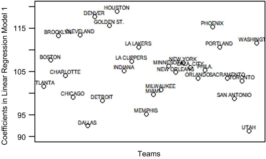
Figure 4 shows that the coefficients of different teams from NBA are in the
range of 90 - 120, and most of teams’ coefficients are near 105. HOUSTON,
DENVER are the strongest teams in that season and DALAS, UTAH are the
weakest teams in that season by virtue of coefficients.
Figure 2. Scatter chart of pre-game Over/Under and actual score totals.
DOI: 10.4236/jss.2021.92013 180 Open Journal of Social SciencesW. P. Di et al.
Figure 3. Part of the matrix 1 for model 1.
Figure 4. Distribution of value of coefficients of each teams.
The plot above shows the strength of each team in the NBA in the 2016-2017
season according to the number of points they scored. Indeed, when incorpo-
rating those coefficients into the model, we would get a partial picture of the
strength of each NBA team. Using L.A. Lakers as the focal point, we want to
compare the actual spread and the odds proposed by Vegas sportsbook.
4.2. Model 2
Now we are considering the model base on the difference between two teams.
Since we filter the data set by keeping the games who have positive difference in
score, then the actual difference should be all greater than 0, and if the point
spreads meet the true results, then most of point spreads should be greater than 0.
Figure 5 shows that the actual score difference is in range of 0 - 50 (because
the points which value of actual score difference is negative have been deleted
all), and the value of difference from prediction is in range of (-20)-25. If the de-
leted data are involved in the scatter chart, the distribution of these remaining
points and existing points are symmetry at the center of (0, 0).
Since we are interested in the points spread instead of Over/Under, if we were
to select two different teams to compare, the coefficient of one team must be
negative. Remember in the Over/Under linear regression model, there is no need
to flip the sign of the coefficient of one team because we are interested in the to-
tal points of two teams. Simply choose L.A. Lakers as the primary predictor, we
DOI: 10.4236/jss.2021.92013 181 Open Journal of Social SciencesW. P. Di et al.
want to be able to show statistically that the point spreads of the Lakers in the
2016-2017 season compared to other teams. There are 3 different conditions of
this model. LA. Lakers can be either team 1, team 2 or didn’t take part in the
game.
LA. Lakers is team 1:
− βi
LA. Lakers is team 2:
+ βi
Lakers didn’t take part in the game:
( β team1 − βlakers ) − ( β team2 − βlakers )
Remember the coefficients mean the strength difference between the team and
Lakers.
For example: if the first team is 2 units better than Lakers and the other is 1
unit better, then we have 2 − 1 = 1, that is: the first team is 1 unit better than the
second, which meets what we expected.
We create another matrix in which L.A. Lakers is the selected team and com-
pare its strength to the league then compare the predict score with the actual
score.
Figure 6 “+1” represent team1 and “−1” represent team 2.
Figure 7 shows the coefficients we got from model 2, for example, the coeffi-
cients for Houston is 12, which means it is 12 units better than Lakers.
Figure 8 shows that using past data and historical odds, the multiple linear
regression model 1 can predict accurately up to 85% of the handicap odds of the
game, and model 2 can predict 75%. The multiple linear regression models are
able to predict and take a correct bet on the final score, score difference and even
the game outcome (Muske & Rawlings, 1993).
Figure 5. Scatter chart of pre-game difference and actual score difference.
DOI: 10.4236/jss.2021.92013 182 Open Journal of Social SciencesW. P. Di et al.
Figure 6. Part of the matrix 2 for model 2.
Figure 7. Team strength compared with LA. Lakers.
Figure 8. Compared predicted score with actual score.
5. Conclusion
The prediction algorithm can be improved by incorporating home field advan-
tage, and other important factors on player performance ensure a more reliable
and accurate prediction, for example, including three-point shooting percentage,
the number of rebounds, and more detailed offensive or defensive data and
finding coefficients for how each variable that affects the result. We can even
collect the individual players’ data so that when there are personnel adjustments
between teams, we can get a new model of team strength. Furthermore, a
head-to-head analysis would provide insight into the interactions among differ-
ent factors affecting performance and what would be the best way to combine
different variables into the predictive power of the predictive algorithm. For
example, while Houston Rockets players score more points than the other teams,
their small-ball style of play generates a high percentage of turnovers, which can
also lead to low quality offensive performance against teams with stellar defenses
such as the Spurs. These observations motivated us to study different ways of
predicting team strengths by combining these different elements of the team and
individuals’ performances. Moreover, another method of analyzing the game of
basketball in aggregate is to look at the designated odds and the corresponding
probability of different teams’ matches. However, this method is often hampered
DOI: 10.4236/jss.2021.92013 183 Open Journal of Social SciencesW. P. Di et al.
by the complex structure of the game and players’ tendencies and strategies.
For R code regarding to this project, see Appendix I.
Conflicts of Interest
The authors declare no conflicts of interest regarding the publication of this
paper.
References
Bhandari, I., Colet, E., Parker, J., et al. (1997). Advanced Scout: Data Mining and Know-
ledge Discovery in NBA Data. Data Mining and Knowledge Discovery 1, 121-125.
https://doi.org/10.1023/A:1009782106822
De Jonge, E., & Van Der Loo, M. (2013). An Introduction to Data Cleaning with R. The
Hague: Statistics Netherlands.
Golec, J., & Tamarkin, M. (1995). Do Bettors Prefer Long Shots Because They Are
Risk-Lovers, or Are They Just Overconfident? Journal of Risk and Uncertainty, 11,
51-64. https://doi.org/10.1007/BF01132730
Humphreys, B. R., Paul, R. J., & Weinbach, A. P. (2013). Consumption Benefits and
Gambling: Evidence from the NCAA Basketball Betting Market. Journal of Economic
Psychology, 39, 376-386. https://doi.org/10.1016/j.joep.2013.05.010
Manner, H. (2016). Modeling and Forecasting the Outcomes of NBA Basketball Games.
Journal of Quantitative Analysis in Sports, 12, 31-41.
https://doi.org/10.1515/jqas-2015-0088
Miljković, D., Gajić, L., Kovačević, A., & Konjović, Z. (2010). The Use of Data Mining for
Basketball Matches Outcomes Prediction. IEEE 8th International Symposium on Intel-
ligent Systems and Informatics, Subotica, 10-11 September 2010, 309-312.
Ahttps://doi.org/10.1109/SISY.2010.5647440
Muske, K. R., & Rawlings, J. B. (1993). Model Predictive Control with Linear Models.
AIChE Journal, 39, 262-287. https://doi.org/10.1002/aic.690390208
Nasseri, H., Sohrabi, M., & Ardil, E. (2008). Solving Fully Fuzzy Linear Systems by Use of
a Certain Decomposition of the Coefficient Matrix. Int. J. Comput. Math. Sci., 3.
Roesser, R. (1975). A Discrete State-Space Model for Linear Image Processing. IEEE
Transactions on Automatic Control, 20, 1-10.
https://doi.org/10.1109/TAC.1975.1100844
Spann, M., & Skiera, B. (2009). Sports Forecasting: A Comparison of the Forecast Accuracy
of Prediction Markets, Betting Odds and Tipsters. Journal of Forecasting, 28, 55-72.
https://doi.org/10.1002/for.1091
DOI: 10.4236/jss.2021.92013 184 Open Journal of Social SciencesW. P. Di et al.
Appendix I: R code
xW. P. Di et al.
results[grep("W", results)]W. P. Di et al.
mm1You can also read