PuckNet: Estimating hockey puck location from broadcast video - arXiv.org
←
→
Page content transcription
If your browser does not render page correctly, please read the page content below
PuckNet: Estimating hockey puck location from broadcast video

                                                              Kanav Vats           William McNally Chris Dulhanty                    Zhong Qiu Lin
                                                                                        David A. Clausi John Zelek
                                                                                                  University of Waterloo
                                                                                                 Waterloo, Ontario, Canada
                                                         {k2vats,wmcnally,chris.dulhanty,zhong.q.lin,dclausi,jzelek}@uwaterloo.ca
arXiv:1912.05107v2 [cs.CV] 13 Apr 2020

                                                                     Abstract
                                              Puck location in ice hockey is essential for hockey ana-
                                              lysts for determining the location of play and analyz-
                                              ing game events. However, because of the difficulty
                                              involved in obtaining accurate annotations due to the
                                              extremely low visibility and commonly occurring oc-
                                              clusions of the puck, the problem is very challeng-
                                              ing. The problem becomes even more challenging in
                                              broadcast videos with changing camera angles. We in-
                                              troduce a novel methodology for determining puck lo-
                                              cation from approximate puck location annotations in
                                              broadcast video. Our method uniquely leverages the ex-
                                              isting puck location information that is publicly avail-          Figure 1: Distribution of some puck locations on the hockey
                                              able in existing hockey event data and uses the corre-            rink. The locations are evenly distributed throughout the ice
                                              sponding one-second broadcast video clips as input to             rink. The red, blue and green circles correspond to the puck
                                              the network. The rationale behind using video as input            locations of shots, dumps and faceoffs respectively.
                                              instead of static images is that with video, the temporal
                                              information can be utilized to handle puck occlusions.
                                              The network outputs a heatmap representing the proba-
                                              bility of the puck location using a 3D CNN based archi-           feasible at the most elite professional level, e.g., the Na-
                                              tecture. The network is able to regress the puck location         tional Hockey League (NHL). Information regarding player
                                              from broadcast hockey video clips with varying cam-               and puck position is therefore inaccessible in most cases. As
                                              era angles. Experimental results demonstrate the capa-            a result, the conventional heuristic approach for evaluating
                                              bility of the method, achieving 47.07% AUC on the test            the effectiveness of team strategies involves analyzing the
                                              dataset. The network is also able to estimate the puck            record of events that occurred during the match (turnover,
                                              location in defensive/offensive zones with an accuracy            shot, hit, face-off, dump, etc.) (Tora, Chen, and Little 2017;
                                              of greater than 80%.                                              Fani et al. 2017).
                                                                                                                   In the NHL, events are recorded on a play-by-play basis
                                                                 Introduction                                   by dedicated statisticians1 . Additionally, third-party hockey
                                                                                                                analytics companies provide more in-depth event informa-
                                         Ice hockey is played by an estimated 1.8 million people
                                                                                                                tion, including a greater number of event types and event
                                         worldwide (IIHF 2018). As a team sport, the positioning
                                                                                                                details, for the NHL and other hockey leagues around the
                                         of the players and puck on the ice are critical to offensive
                                                                                                                world. Each event is linked with a game-clock timestamp (1-
                                         and defensive strategy (Thomas 2006). Currently, practical
                                                                                                                second resolution), and an approximate location where the
                                         methods for tracking the position of each player and the
                                                                                                                event occurred on the rink. Generally speaking, the event lo-
                                         puck for the full duration of a hockey match are limited.
                                                                                                                cation corresponds to the approximate location of the puck.
                                         Advances in computer vision have shown promise in this
                                                                                                                Therefore, there exists an expansive knowledgebase of ap-
                                         regard (Lu, Okuma, and Little 2009; Pidaparthy and Elder
                                                                                                                proximate puck location information that has, until now, not
                                         2019), but ultimately remain in the developmental phase. As
                                                                                                                been exploited. To this end, this paper explores the follow-
                                         an alternative, radio-frequency identification is currently be-
                                                                                                                ing idea: can we leverage existing hockey event annotations
                                         ing explored for player and puck tracking (Cavallaro 1997;
                                                                                                                and corresponding broadcast video to predict the location
                                         Gulitti 2019), but may only be financially and logistically
                                                                                                                   1
                                         Copyright c 2020, Association for the Advancement of Artificial             Play-by-play event data is publicly available for all NHL
                                         Intelligence (www.aaai.org). All rights reserved.                      games at NHL.com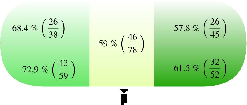
for computation. The puck locations are evenly distributed
throughout the ice rink as can be seen from Figure 1. The
dataset is split such that 80% of the data is used for training,
10% for validation and 10% for testing.
Experiment
We use the 18 layer R(2+1)D (Tran et al. 2018) network
pretrained on the Kinetics dataset (Kay et al. 2017) as a
Figure 2: Illustration of the scaling transformation used to backbone for regressing the puck location from video. The
transform the puck annotation from the ice rink coordinates input to the network consists of 16 video frames {Ii ∈
to the heatmap coordinates. For training, the annotations are R3×256×256 | i ∈ [1, .., 16]} sampled from a one second
transformed from the ice rink coordinates to the heatmap video clip. The 16 frames are sampled from a uniform dis-
coordinates, whereas, predicated heatmap is transformed to tribution. For preprocessing, the image frame RBG pixel
ice-rink coordinates for inference. values are scaled to the [0, 1] range and normalized by the
Kinetics dataset mean and standard deviation. The features
maps obtained from the 9th layer of the R(2+1)D network
of the puck on the ice? is fed into two RegressionBlocks illustrated in Figure 4. The
Using a relatively small dataset of hockey events contain- first five layers of the R(2+1)D network are kept frozen dur-
ing approximate puck locations (distribution shown in Fig- ing training in order to reduce the computational cost and
ure 1), we use a 3D CNN to predict the puck position in the maintain a batch size of 10 on a single GPU machine. Each
rink coordinates using the corresponding 1-second broadcast regression block consists of a 3D convolutional layer, batch
video clips as input. As such, the 3D CNN is tasked with si- normalization and ReLU non-linearity. The final output of
multaneously (1) localizing the puck in RGB video and (2) the network is a two-dimensional heatmap h ∈ R64×64 rep-
learning the homography between the broadcast camera and resenting the probability distribution of the puck location.
the static rink coordinate system. To our best knowledge, this We chose a heatmap based approach instead of directly re-
represents a novel computer vision task that shares few simi- gressing the puck coordinates in order to account for the un-
larities with any existing tasks. Drawing inspiration from the certainty in the ground truth annotations. The overall net-
domain of human pose estimation, we model the approxi- work architecture is illustrated in Figure 3 and Table 1. The
mate spatial puck location using a 2D Gaussian, as shown in ground truth heatmap consists of a Gaussian with mean µ
Figure 2. equal to the ground truth puck location and standard devia-
tion σ. Mean squared error (MSE) loss between the ground
Background truth and predicted heatmap is minimized during training.
Pidaparthy and Elder (2019) proposed using a CNN to The size of the NHL hockey rink is 200f t × 85f t. In
regress the puck’s pixel coordinates from single high- order to predict a 64 × 64 dimensional square heatmap, a
resolution frames collected via a static camera for the pur- scaling transformation τ : R200×85 → R64×64 is applied
pose of automated hockey videography. Estimating the puck to the ground truth puck annotations in rink coordinates
location from a single frame is a challenging task due to while training. Let hmap width and hmap height denote
the relatively small size of the puck compared to the frame, the output heatmap width and height respectively. The trans-
occlusions from hockey sticks, players, and boards, and the formation matrix is given by:
significant motion blur caused by high puck velocities. Fur- hmap width
0 0
thermore, their method was not based on existing data and 200
τ = hmap height
thus required extensive data collection and manual annota- 0 85 0
tion. 0 0 1
Remarking that humans can locate the puck position from During testing, inverse transformation τ −1 is applied to con-
video with the help of contextual cues and temporal infor- vert back to the rink coordinates. This process is illustrated
mation, our method incorporates temporal information in the in Figure 2.
form of RGB video to help localize the puck. Additionally, We use the Adam optimizer with an initial learning rate
our method differs from Pidaparthy and Elder in that we use of .0001 with a batch size of 10. We use the Pytorch 1.3
puck location information obtained from existing hockey framework on an Nvidia GTX 1080Ti GPU.
event data, and directly learn the camera-rink homography
instead of using a manual calibration. Results and Discussion
Accuracy Metric
Methodology
A test example is considered to be correctly predicted at a
Dataset tolerance t feet if the L2 distance between the ground truth
The dataset consists of 2716, 60 fps broadcast NHL clips puck location z and predicted puck location z0 is less than t
with an original resolution of 1280 × 720 pixels of one feet. That is ||z − z0 ||2 < t. Let φ(t) denote the percentage
second each with the approximate puck location annotated. of examples in the test set with correctly predicted position
The videos are resized to a dimension of 256 × 256 pixels puck position at a tolerance of t. We define the accuracy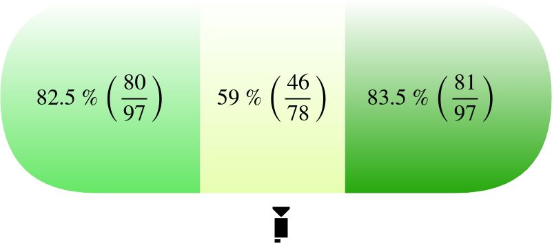
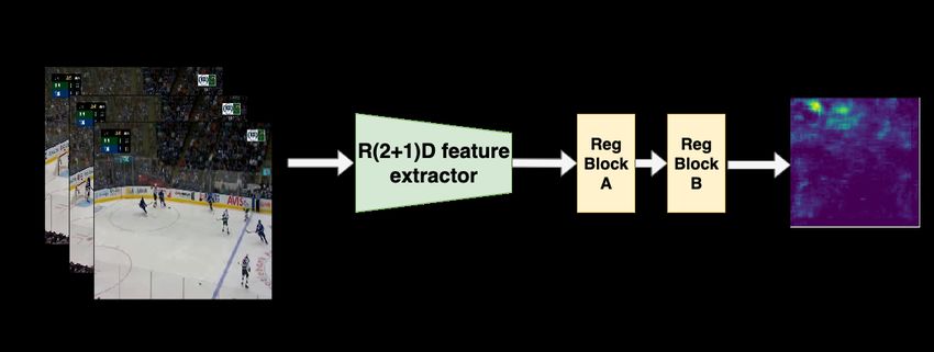
Figure 3: The overall network architecture. Input tensor of dimension b × 16 × 3 × 256 × 256 (b denotes the batch size)
is input into the R(2+1)D feature extractor consisting of the first nine layers of the R(2+1)D network. The feature extractor
outputs b × 8 × 128 × 64 × 64 tensor representing the intermediate features. The intermediate features are finally input into two
regression blocks. The first regression block(Reg Block A) outputs a b × 2 × 32 × 64 × 64 tensor while the second regression
block outputs the final predicted heatmap.

                                                                   Figure 5: Overall AUC for the best performing model with
                                                                   random sampling and σ = 25.
Figure 4: Illustration of the regression block applied after
the R(2+1)D network backbone. The input and outputs are
5D tensors where b, c, t, w and h denote batch size, number        Table 1: Network architecture. k,s and p denote kernel di-
of channels, temporal dimension, width and height of the           mension, stride and padding respectively. Chi and Cho and
                                 0           0
feature map respectively. Here c < x and t < t since the           b denote the number of channels going into and out of a
number of channels and timesteps have to be reduced so that        block and batch size respectively.
                                                                                    Input b × 16 × 3 × 256 × 256
a single heatmap can be generated.
                                                                                           Feature extractor
                                                                                  First 9 layers of R(2+1)D network
                                                                                              RegBlock A
metric as the area under the curve (AUC) φ(t) at tolerance                                      Conv3D
of t = 5 feet to t = 50 feet.                                                           Chi = 128, Cho = 32
                                                                                 (k = 4 × 1 × 1, s = 4 × 1 × 1, p = 0)
Discussion                                                                                  Batch Norm 3D
                                                                                                 ReLU
Figure 5 shows the variation of overall accuracy with toler-                                  RegBlock B
ance t for the best performing model trained with σ = 25.                                       Conv3D
The accuracy increases almost linearly reaching ∼ 60% ac-                                Chi = 32, Cho = 1
curacy for t = 30 feet. The AUC score for the model is                           (k = 2 × 1 × 1, s = 2 × 1 × 1, p = 0)
47.07 %. Figure 6 shows the accuracy vs tolerance plot for                                  Batch Norm 3D
the σ = 25 model, in the horizontal(X) and vertical(Y) di-                                       ReLU
rections separately. The model is able to locate the puck                                Output b × 64 × 64
position with the highest accuracy in Y(vertical) direction
reaching an accuracy of ∼ 65% at a tolerance of t = 15 feet.
This is because the vertical axis is more or less always vis-      horizontal(X) direction since the camera pans horizontally
ible in the camera field of view. This cannot be said for the      and hence, the models has to learn the viewpoint changes.
Figure 8: Zone-wise accuracy with offensive and defensive
zones further split into two. The figure represents the hockey
rink with the text in each zone represents the percentage of
test examples predicted correctly in that zone. The position
Figure 6: The accuracy curves corresponding to the best per- of the camera is at the bottom.
forming model.
Table 3: Comparison between uniform and random sampling
settings. Random sampling outperforms uniform sampling
because it acts as a form of data augmentation.
Sampling σ AUC(overall) AUC(X) AUC(Y)
Random 20 45.80 57.31 76.66
Constant interval 20 36.55 49.24 71.41
Conclusion and Future Work
Figure 7: Zone-wise accuracy. The figure represents the
We have presented a novel method to locate the approximate
hockey rink with the text in each zone represents the per-
puck position from video. The model can be used to know
centage of test examples predicted correctly in that zone.
the zone in which the puck was present at a particular mo-
The position of the camera is at the bottom.
ment in time, which can be of practical significance to know
the exact location of play and as a prior information for rec-
Table 2: AUC values for different values of σ. ognizing game events. The results obtained are preliminary
σ AUC(overall) AUC(X) AUC(Y) and in the future more cues such as player detections, player
10 36.85 48.84 72.25 trajectories on ice and optical flow can be taken into account
15 42.51 53.86 77.12 to obtain more accurate results. It would also be interesting
20 45.80 57.31 76.66 to apply the proposed methodology in sports such as soccer.
25 47.07 58.85 76.78
30 42.86 54.23 76.76 Acknowledgment
This work was supported by Stathletes through the Mitacs
Accelerate Program and Natural Sciences and Engineering
Table 2 shows the variation of AUC for different val- Research Council of Canada (NSERC).
ues of σ. The highest AUC score achieved is correspond-
ing to σ = 25 (47.07 %). A lower value of σ results in
a lower accuracy. A reason for this can be that with lower References
σ, the ground truth Gaussian distribution becomes more [Cavallaro 1997] Cavallaro, R. 1997. The FoxTrax hockey
rigid/peaked, which makes learning difficult. For a value of puck tracking system. IEEE Computer Graphics and Appli-
σ > 25, the accuracy again lowers because the ground truth cations 17(2):6–12.
Gaussian becomes very spread out, which lowers accuracy [Fani et al. 2017] Fani, M.; Neher, H.; Clausi, D. A.; Wong,
on lower tolerance levels. A.; and Zelek, J. 2017. Hockey action recognition via in-
Two kinds of sampling techniques were investigated: 1) tegrated stacked hourglass network. In Proceedings of the
Random sampling from a uniform distribution 2) Constant IEEE Conference on Computer Vision and Pattern Recogni-
interval sampling at an interval of 4 frames. Random sam- tion Workshops, 29–37.
pling outperforms uniform sampling because it acts as a
[Gulitti 2019] Gulitti, T. 2019. NHL plans to deploy Puck
form of data augmentation. This is shown in Table 3.
and Player Tracking technology next season.
Figure 7 shows the zone-wise accuracy of the model. A
prediction is labelled as correct if it lies in the same zone as [IIHF 2018] IIHF. 2018. Survey of Players. Avail-
the ground truth. The model shows good performance in the able online: https://www.iihf.com/en/static/5324/survey-of-
offensive and defensive zones with an accuracy greater than players.
80%. The model maintains reasonable performance when [Kay et al. 2017] Kay, W.; Carreira, J.; Simonyan, K.; Zhang,
the defensive and offensive zones are further split into two B.; Hillier, C.; Vijayanarasimhan, S.; Viola, F.; Green, T.;
(Figure 8). Back, T.; Natsev, A.; Suleyman, M.; and Zisserman, A.2017. The kinetics human action video dataset. ArXiv abs/1705.06950. [Lu, Okuma, and Little 2009] Lu, W.-L.; Okuma, K.; and Little, J. J. 2009. Tracking and recognizing actions of mul- tiple hockey players using the boosted particle filter. Image and Vision Computing 27(1-2):189–205. [Pidaparthy and Elder 2019] Pidaparthy, H., and Elder, J. 2019. Keep your eye on the puck: Automatic hockey videog- raphy. In 2019 IEEE Winter Conference on Applications of Computer Vision (WACV), 1636–1644. IEEE. [Thomas 2006] Thomas, A. C. 2006. The impact of puck possession and location on ice hockey strategy. Journal of Quantitative Analysis in Sports 2(1). [Tora, Chen, and Little 2017] Tora, M. R.; Chen, J.; and Lit- tle, J. J. 2017. Classification of puck possession events in ice hockey. In 2017 IEEE Conference on Computer Vision and Pattern Recognition Workshops (CVPRW), 147–154. IEEE. [Tran et al. 2018] Tran, D.; Wang, H.; Torresani, L.; Ray, J.; LeCun, Y.; and Paluri, M. 2018. A closer look at spa- tiotemporal convolutions for action recognition. In 2018 IEEE/CVF Conference on Computer Vision and Pattern Recognition, 6450–6459.
You can also read