Social networks predict the life and death of honey bees - Nature
←
→
Page content transcription
If your browser does not render page correctly, please read the page content below
ARTICLE
                  https://doi.org/10.1038/s41467-021-21212-5                  OPEN

                  Social networks predict the life and death of honey
                  bees
                  Benjamin Wild 1,8 ✉, David M. Dormagen 1,8, Adrian Zachariae2,8, Michael L. Smith                                           3,4,5,

                  Kirsten S. Traynor 1,6, Dirk Brockmann2,7, Iain D. Couzin 3,4,5 & Tim Landgraf 1 ✉
1234567890():,;

                  In complex societies, individuals’ roles are reflected by interactions with other conspecifics.
                  Honey bees (Apis mellifera) generally change tasks as they age, but developmental trajec-
                  tories of individuals can vary drastically due to physiological and environmental factors. We
                  introduce a succinct descriptor of an individual’s social network that can be obtained without
                  interfering with the colony. This ‘network age’ accurately predicts task allocation, survival,
                  activity patterns, and future behavior. We analyze developmental trajectories of multiple
                  cohorts of individuals in a natural setting and identify distinct developmental pathways and
                  critical life changes. Our findings suggest a high stability in task allocation on an individual
                  level. We show that our method is versatile and can extract different properties from social
                  networks, opening up a broad range of future studies. Our approach highlights the rela-
                  tionship of social interactions and individual traits, and provides a scalable technique for
                  understanding how complex social systems function.

                  1 Department of Mathematics and Computer Science, Freie Universität Berlin, Berlin, Germany. 2 Robert Koch Institute, Berlin, Germany. 3 Department of

                  Collective Behaviour, Max Planck Institute of Animal Behavior, Konstanz, Germany. 4 Centre for the Advanced Study of Collective Behaviour, University of
                  Konstanz, Konstanz, Germany. 5 Department of Biology, University of Konstanz, Konstanz, Germany. 6 Global Biosocial Complexity Initiative, Arizona State
                  University, Tempe, FL, USA. 7 Institute for Theoretical Biology, Humboldt University Berlin, Berlin, Germany. 8These authors contributed equally: Benjamin
                  Wild, David M. Dormagen, Adrian Zachariae. ✉email: b.w@fu-berlin.de; tim.landgraf@fu-berlin.de

                  NATURE COMMUNICATIONS | (2021)12:1110 | https://doi.org/10.1038/s41467-021-21212-5 | www.nature.com/naturecommunications                                1
ARTICLE                                                                   NATURE COMMUNICATIONS | https://doi.org/10.1038/s41467-021-21212-5

I
    n complex systems, intricate global behaviors emerge from the             behavior57. While honey bees are well known for their elaborate
    dynamics of interacting parts. Within animal groups, studying             social signals (e.g., waggle dance, shaking signal, stop signal58–60),
    interactions helps to elucidate the individuals’ functions1–4.            they also exchange information through food exchange, anten-
Descriptors of individuals derived from social interaction networks           nation, or simple colocalization61,62. However, identifying an
have been used to investigate, for example, pair bonding5, inter-             individual bee’s role in a colony based on its characteristic pat-
group brokering6, offspring survival7, cultural spread8,9, policing           terns of interaction remains challenging, particularly with large
behavior10, leadership11–13, organization of food retrieval14, the            numbers of individuals and multiple modes of interaction.
ability to affect behavioral change15, and behavior during famine                In this work, we investigate the relationship between an indi-
events16. As our ability to collect detailed social network data              vidual’s social network and its lifetime role within a complex
increases, so too does our need to develop tools for understanding            society. We developed a tracking method for unbiased long-term
the significance and functional consequences of these networks17.              assessment of a multitude of interaction types among thousands
   Social insects are an ideal model system to study the rela-                of individuals of an entire honey bee colony with a natural age
tionship between social interactions and individual roles because             distribution. We introduce a low-dimensional descriptor, network
task allocation has long been hypothesized to arise from inter-               age, that allows us to compress the social network of all indivi-
actions18–20. The relationship of individual roles within the col-            duals in the colony into a single number per bee per day. Network
ony and the social network; however, is not well understood.                  age, and therefore the social network of a bee, captures the
Individuals, for example, can modify their behavior based on                  individual’s behavior and social role in the colony and allows us
nestmate interaction21–24, and interactions change depending on               to predict task allocation, mortality, and behavioral patterns such
where and with whom individuals interact14,22,25,26. These studies            as velocity and circadian rhythms. Following the developmental
typically target specific types of interactions (e.g., food exchange),         trajectories of individual honey bees and cohorts that emerged on
specific roles within task allocation (e.g., foraging), or specific             the same day reveals clusters of different developmental paths,
stimuli within the nest (e.g., brood), but an automatic observation           and critical transition points. In contrast to these distinct clusters
system could capture behaviors and interactions within a colony               of long-term trajectories, we find that transitions in task alloca-
more comprehensively and without human bias. Measuring the                    tion are fluid on an individual level. We show that the task
multitude of social interactions and their effect on behavior, and the        allocation of individuals in a natural setting is stable over long
social networks over the lifetime of individuals without interfering          periods, allowing us to predict a worker’s task better than
with the system (e.g., by removing individuals) is an open problem.           biological age up to 1 week into the future.
   In honey bees, task allocation is characterized by temporal
polyethism27–29, where workers gradually change tasks as they
age: young bees care for brood in the center of the nest, while old           Results
bees forage outside30,31. Previous works often used few same-aged             What is network age? To obtain the social network structure
cohorts resulting in an unnatural age distribution27,28,30,32. The            over the lifetime of thousands of bees, we require methods that
developmental trajectory of individuals can, however, vary dras-              will track the tasks and social interactions of many individuals
tically due to internal factors (i.e., genetics, ovary size, sucrose          over consecutive days. We video recorded a full colony of indi-
responsiveness33–39), nest state (i.e., amount of brood, brood age,           vidually marked honey bees (Apis mellifera) at 3 Hz for 25 days
food stores40–42), and the external environment (i.e., season,                (from 1 August 2016 to 25 August 2016) and obtained continuous
resource availability, forage success43–46). These myriad influ-               trajectories for all individuals in the hive63,64. We used a two-
ences on maturation rate are difficult to disentangle, but all drive           sided single-frame observation hive with a tagged queen and
the individual’s behavior and task allocation. Due to the spatial             started introducing individually tagged bees into the colony
organization of honey bee colonies, task changes also result in a             ~1 month before the beginning of the focal period (see “Methods:
change of location, with further implications on the cues that                ‘Recording setup, data extraction, and preprocessing’” for details).
workers encounter31. How and when bees change their allocated                 To ensure that no unmarked individuals emerged inside the hive,
tasks in a natural setting has typically been assessed through                we replaced the nest substrate regularly (approx. every 21 days).
destructive sampling (e.g., for measuring hormone titers of                   In total, we recorded 1920 individuals aged from 0 days to
selected individuals), but understanding how all these factors                8 weeks.
combine would ideally be done in an undisturbed system.                          A worker’s task and the proportion of time she spends in
   With the advent of automated tracking, there has been renewed              specific nest areas are tightly coupled in honey bees31. We
interest in how interactions change within colonies47,48, how                 annotated nest areas associated with specific tasks (e.g., brood area
spatial position predicts task allocation49, and how spreading                or honey storage) for each day separately (see “Methods: ‘Nest
dynamics occur in social networks32. Despite extensive work on                area mapping and task descriptor’”), as they can vary in size and
the social physiology of honey bee colonies50, few works have                 location over time65. We then use the proportion of time an
studied interaction networks from a colony-wide or temporal                   individual spends in these areas throughout a day as an estimate of
perspective32,51. While there is considerable variance in task                her current tasks.
allocation, even among bees of the same age, it is unknown to                    We calculated daily aggregated interaction networks from
what extent this variation is reflected in the social networks. In             contact frequency, food exchange (trophallaxis), distance, and
large social groups, like honey bee colonies, typically only a subset         changes in movement speed after contacts (see “Methods: ‘Social
of individuals are tracked, or tracking is limited to short time              networks’”). These networks contain the pairwise interactions
intervals28,47,52,53.                                                         between individuals over time. For each day and interaction type,
   Tracking an entire colony over a long time would allow one to              we extract a compact representation that groups bees together with
investigate the stability of task allocation. Prior research has              similar interaction patterns, using spectral decomposition66,67. We
shown that during each life stage, an individual spends most of its           then combine each bees’ daily representations of all interaction
time in a specific nest region31,54, interacting with nestmates, but           types and map them to a scalar value (network age) that best
with whom they interact may depend on more than location                      reflects the fraction of time spent in the task-associated areas using
alone (e.g., previous interactions, or the genetic diversity within           CCA (canonical-correlation analysis; refs. 68,69). Note that network
the colony55,56). Social interactions permit an exchange of                   age is solely a representation of the social network and not of
information and can have long-term effects on an individual’s                 location; the fraction of time spent in the task-associated areas is

2                 NATURE COMMUNICATIONS | (2021)12:1110 | https://doi.org/10.1038/s41467-021-21212-5 | www.nature.com/naturecommunications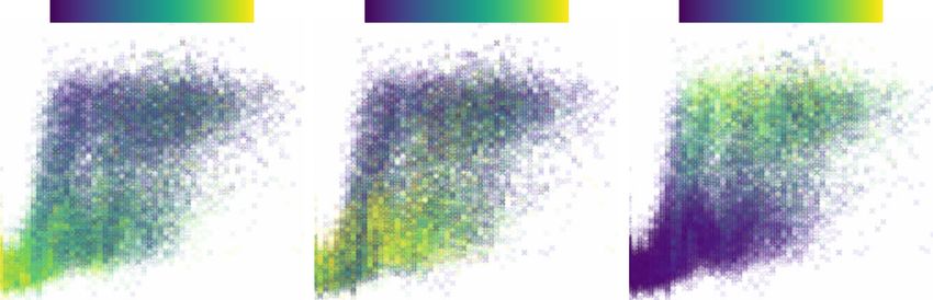
NATURE COMMUNICATIONS | https://doi.org/10.1038/s41467-021-21212-5                                                                       ARTICLE

Fig. 1 Network age, a one-dimensional descriptor of an individual’s role within the colony, based on an individual’s interaction pattern. Using the
BeesBook automated tracking system, we obtain lifetime tracking data for individuals (a). These tracks are used to construct multiple weighted social
interaction networks (b). We aggregate daily networks (c) to then extract embeddings that group bees together with similar interaction patterns, using
spectral decomposition (d). Finally, we use a linear transformation (e; CCA canonical-correlation analysis) that maximizes correlation with the fraction of
time spent in different nest areas (f) to compress them into a single number per day called “network age” (g).

only used to select which information to extract from the social                 Table 2 and see “Methods: ‘Statistical comparison of models’” for
networks (e.g., by assigning higher importance to proximity                      details). Network age provides a better separability of time spent
contacts, see Supplementary Note 1.1). Network age can still                     in task-associated nest areas than biological age (Fig. 2a, example
represent an individual’s location, but only if this information is              cohort in Fig. 2c, Supplementary Note 1.2 for all cohorts).
inherently present in the social networks. Network age thus                      Network age correlates with the location because of the inherent
compresses millions of data points per individual and day (1919                  coupling between tasks and nest areas. Still, it is not a direct
potential interaction partners, each detected 127,501 ± 50,340 times             measure of location: bees with the same network age can exhibit
on average per day, with four different interaction types) into a                different spatial distributions and need not directly interact (see
single number that represents each bee’s daily position in the                   Supplementary Note 2.1).
multimodal temporal interaction network. Since CCA is applied                       While we can improve the predictive power of network age by
over the 25 days of the focal period, network age can only represent             extracting a multidimensional descriptor instead of a single
interaction patterns that are consistent over time. See Fig. 1 for an            value (see “Methods: ‘Network age: from networks to spectral
overview and “Methods: ‘Network age: from networks to spectral                   embeddings to CCA’ and ‘Task prediction models and boot-
embeddings to CCA’” for a detailed description of the methods.                   strapping’” for details), the improvements for additional dimen-
   Network age is a unitless descriptor. We scale it such that 90%               sions are marginal compared to the difference in predictiveness
of the values are between 0 and 40 to make it intuitively                        between the first dimension of network age and biological age (see
comparable to a typical lifespan of a worker bee during summer,                  Supplementary Table 2). This implies that a one-dimensional
and because biological age is commonly associated with task                      descriptor captures most of the information from the social
allocation in honey bees. This scaling can be omitted for systems                networks that are relevant to the individuals’ location preferences
where behavior is not coupled with biological age.                               and therefore their tasks.
                                                                                    We experimentally demonstrated that network age robustly
                                                                                 captures an individual’s task by setting up sucrose feeders and
Network age correctly identifies task allocation. Because of the                  identifying workers that foraged at the feeders (known foragers,
inherent coupling of tasks and locations in a honey bee colony,                  N = 40, methods in “Methods: ‘Forager groups’ experiment’”).
we expect a meaningful measure of social interaction patterns to                 We then compared the biological ages of these known nectar
be correlated with the individual’s spatial preferences. We quantify             foragers to their network ages. We made these two quantities
to what extent network age captures this correlation by using                    comparable by z-transforming them because they do not have the
multinomial regression to predict the fraction of time each bee                  same unit of measure. As expected, foragers exhibited a high
spends in the annotated nest areas (see “Methods: ‘Task prediction               biological age and a high network age, whereas biological age
models and bootstrapping’”). Note that while we also used these                  exhibited significantly larger variance than network age (Fig. 2b;
spatial preferences to select which information to extract from the              Levene’s test71, performed on z-transformed values: p ≪ 0.001,
interaction networks, it is not certain whether the spatial infor-               N = 200). Indeed, while we observed a forager as young as
mation is contained in the social network in the first place, and                 12 days old, that individual had a network age of 25.5,
how well a single dimension can capture it. Furthermore, the                     demonstrating that network age more accurately reflected her
social network structure could vary over many days with changing                 task than her biological age (z-transformed values: biological age
environmental influences, preventing the extraction of a stable                   −0.46; network age 0.61).
descriptor. The regression analysis allows us to compare different                  Tagging an entire honey bee colony is laborious. However, by
variants of network age to biological age as a reference.                        sampling subsets of bees, we find that network age is still a viable
   To evaluate the regression fit, we use McFadden’s pseudo R2                    metric, even when only a small proportion of individuals are
scores R2McF 70. Network age is twice as good as biological age at               tagged and tracked. With only 1% of the bees tracked, network
predicting the individuals’ location preferences, and therefore                  age is still a good predictor of task (median R2McF ¼ 0:516, 95% CI
their tasks (network age: median R2McF ¼ 0:682, 95% confidence                    [0.135, 0.705], N = 128) while increasing the number of tracked
interval (CI) [0.678, 0.687]; biological age: median R2McF ¼ 0:342,              individuals to 5% of the colony results in an R2McF value
95% CI [0.335, 0.349]; 95% CI of effect size [0.332, 0.348], N =                 comparable to the fully tracked colony (5% of colony tracked:
128; likelihood ratio χ2 test p ≪ 0.001, N = 26403, Supplementary                median R2McF ¼ 0:650, 95% CI [0.578, 0.705], N = 128; whole

NATURE COMMUNICATIONS | (2021)12:1110 | https://doi.org/10.1038/s41467-021-21212-5 | www.nature.com/naturecommunications                                 3
ARTICLE NATURE COMMUNICATIONS | https://doi.org/10.1038/s41467-021-21212-5
Fig. 2 Network age is an accurate descriptor of task allocation. a The proportion of time spent on task-associated locations in relation to biological age
and network age with each cross representing one individual on one day of her life. For a given value on the y-axis (network age) colors are more consistent
than for a given value on the x-axis (biological age). b Z-transformed age distributions for known foragers visiting a feeder (N = 40 observed individuals).
The variance in biological age is greater than the variance in network age (boxes: center dot; median; box limits; upper and lower quartiles; whiskers, 1.5×
interquartile range). Corresponding biological ages are also shown on the right y-axis (original biological age: 34.2 ± 7.9; original network age: 38.3 ± 4.6;
mean ± standard deviation). c Spatial distributions of an example cohort over time (bees emerged on 29 July 2016, 64 individuals over 25 days), grouped
by biological age (top row) versus network age (bottom row). Note how network age more clearly delineates groups of bees than biological age, with bees
transitioning from the brood nest (center of the comb), to the surrounding area, to the dance floor (lower left area). The shaded areas depict density
percentiles (brightest to darkest: 99%, 97.5%, 95%, 80%, 70%, 20%).
colony tracked: median R2McF ¼ 0:682, 95% CI [0.678, 0.687], We attribute the split on the population level to distinct
N = 128; see Supplementary Note 2.2). Similarly, we find that an patterns of individual development. Clustering the time series of
approximation of network age can be calculated without network ages over the lives of bees identifies distinct develop-
annotated nest areas: Network age can be extracted in an mental paths within same-aged cohorts. We set the number of
unsupervised manner using principal component analysis (PCA) clusters to three as this is the minimum number of clusters that
on the spectral embeddings of the different interaction type separates an early and a late transition from low to high network
matrices (median R2McF ¼ 0:646, 95% CI [0.641, 0.650], N = 128, age in all tested cohorts (see “Methods: ‘Network age transition
see “Methods: ‘Network age: unsupervised variant using PCA’”). clustering’” for further details). In the cohort that emerged on
1 August 2016, the first developmental cluster (blue, Fig. 3b)
rapidly transitions to a high network age (likely corresponding to
Developmental changes over the life of a bee. Network age foraging behavior) after only 11 days. The second cluster (orange)
reveals differences in interaction patterns and task allocation transitions at ~21 days of biological age, while bees in the third
among same-aged bees (Fig. 3a). After around 6 days of biological cluster (green) remain at a lower network age throughout the
age, the network age distribution becomes bimodal (see “Meth- focal period. We see similar splits in developmental trajectories
ods: ‘Quantifying when bees first split into distinct network age for all cohorts, although the timing of these transitions varies (see
modes’”). Bees in the functionally old group (high network age) “Methods: ‘Network age transition clustering’” for additional
spend the majority of their time on the dance floor, whereas cohorts). Such divergence in task allocation has been previously
same-aged bees in the functionally young group (low network shown in bees; factors that accelerate a precocious transition to
age) are found predominantly in the honey storage area (Fig. 3a). foraging include hormone titers72, genotype35, and physiology,
Transitions from high to low network age are a rare occurrence in especially the number of ovarioles73, and sucrose response
our colony (see Supplementary Note 2.3). threshold74.
4 NATURE COMMUNICATIONS | (2021)12:1110 | https://doi.org/10.1038/s41467-021-21212-5 | www.nature.com/naturecommunicationsNATURE COMMUNICATIONS | https://doi.org/10.1038/s41467-021-21212-5 ARTICLE Fig. 3 Network age reveals distinct developmental paths. a Left: The median of network ages over biological ages for all individuals that lived more than 11 days split by a threshold on the age of 11 (T = 23.07, calculated using Otsu’s method84.The upper line contains all bees that fall above this threshold (N = 832), the lower contains all bees below that threshold (N = 563). The shaded areas depict 20%, 40%, 60% data intervals. We observe a split in network age corresponding to different tasks: The upper heatmap (network age 30–40, biological age 20–30, 577 bees, 857,283 data points) corresponds to the dance floor, while the lower heatmap (network age 5–15, biological age 20–30, 381 bees, 742,622 data points) borders between the dance floor and brood nest. Right: The mean fraction of time a bee with a given network age spends on our annotated regions throughout a day. b Lines depict the network age of individual bees of a same-aged cohort with the colors indicating clusters of their network age over time. Boxes summarize bees belonging to each cluster for a given day (center line, median; box limits, upper and lower quartiles; whiskers, 1.5× interquartile range). c Heatmaps showing the spatial distribution of bees in the developmental cluster 2 (orange) from 19 August 2016 to 24 August 2016. The smooth transition in network age (orange in line plot, b) from one mode to another corresponds to a smooth transition in spatial location (heatmaps, c). The shaded areas depict density percentiles (brightest to darkest: 99%, 97.5%, 95%, 80%, 70%, 20%). The transition from low to high network age over multiple days (median R = 0.612 95% CI = [0.199, 0.982], see “Methods: is characterized by a gradual shift in the spatial distribution (see ‘Repeatability’” for details), indicating task stability over multiple example in Fig. 3c), highlighting that an individual’s task changes days. Both findings (gradual change over a few days and high gradually. The network age of most bees is highly repeatable repeatability) are consistent with the dynamics of the underlying NATURE COMMUNICATIONS | (2021)12:1110 | https://doi.org/10.1038/s41467-021-21212-5 | www.nature.com/naturecommunications 5
ARTICLE                                                                     NATURE COMMUNICATIONS | https://doi.org/10.1038/s41467-021-21212-5

physiological processes, such as vitellogenin and juvenile                      predicts other behaviors better than biological age, including an
hormone, that influence task allocation and the transition to                    individual’s impending death (network age: median R2 = 0.165,
foraging75.                                                                     95% CI [0.158, 0.172], versus biological age: median R2 = 0.064,
                                                                                95% CI [0.059, 0.068]; 95% CI of effect size [0.037, 0.039], N =
Network age predicts an individual’s behavior and future role                   128, likelihood ratio χ2 test p ≪ 0.001, N = 26,403). Biologically
in the colony. Network age predicts task allocation (i.e., in what              young but network-old bees have a significantly higher
part of the nest individuals will be) up to 10 days into the future.            probability of dying within a week (80.6% N = 139) than do
Knowing the network age of a bee today allows a better prediction               biologically old but network-young bees (42.1% N = 390; χ2test of
of the task performed by that individual next week than her                     independence p ≪ 0.001 N = 529; see Supplementary Note 3.1 for
biological age informs about her current tasks (Fig. 4c, binomial               details). This is likely because a biologically young bee with a high
test, p ≪ 0.001, N = 55390, 95% CI of effect size [0.055, 0.090],               network age, that is, a bee that starts to forage earlier in life and
N = 128, see “Methods: ‘Future predictability’” for details). We                faces more perils imposed by the outside world, is more likely to
confirm that this is only partially due to network age being                     die than a bee of the same age with a low network age. This
repeatable (see “Methods: ‘Future predictability’”). We do note,                finding is consistent with previous work showing increased
however, that our ability to predict the future tasks of a young bee            mortality with precocious foraging76,77.
is limited, especially before cohorts split into high and low net-                 We measure movement patterns of individual bees such as
work age groups (Fig. 3a). This limitation hints at a critical                  daily and nightly average speed, the circadian rhythm, and the
developmental transition point in their lives, an attractive area for           time of an individual’s peak activity. While these properties are
future study.                                                                   related to task allocation due to the diurnal nature of foraging,
   We explicitly optimized network age to be a good predictor of                they are not direct measures of an individual’s location. Network
task-associated locations. However, we find that network age                     age also captures these movement patterns better than biological

Fig. 4 Network age can be used to predict other properties, such as mortality and circadian rhythms. It also predicts an individual’s future task
allocation. a An individual’s mortality on the next day based on her age (x-axis show original and z-transformed biological age and z-transformed network
age). Bees with a low network age have lower mortality than biologically young bees; bees with a high network age have higher mortality than biologically
old bees (shaded areas: 95% bootstrap confidence intervals for the regression estimates). b Network age can be used to predict task allocation and future
behaviors. Network age predicts the task of an individual 7 days into the future better than biological age predicts the individual’s task the same day (blue
dotted line). Each box comprises N = 12 scores from models with N = 12 days of training data (center line, median; box limits, upper and lower quartiles;
whiskers, 1.5× interquartile range; points, outliers). c Selected properties mapped for network age over biological age with each cross representing one
individual on one day of her life. Note that for a given value on the y-axis (network age) colors are more consistent than for a given value on the x-axis
(biological age).

6                   NATURE COMMUNICATIONS | (2021)12:1110 | https://doi.org/10.1038/s41467-021-21212-5 | www.nature.com/naturecommunications
NATURE COMMUNICATIONS | https://doi.org/10.1038/s41467-021-21212-5 ARTICLE
age (likelihood ratio χ2 test p ≪ 0.001, N = 26403, see Supple- interactions are inherently coupled in honey bees. However, we
mentary Table 1b for 95% CI of effect sizes). show that network age is more than just a representation of
To investigate whether network age is a good predictor of location: Bees with the same network age do not necessarily share
future task allocation and behavior only because it captures the a location in the nest, and the time spent in task-associated
spatial information contained in the social network, we repeat the locations is less predictive of an individual’s current and future
analyses above using the time spent in task-associated locations as behavior than network age. In addition, we calculate a variant of
independent variables. We find that network age, even though it network age that is not guided by auxiliary spatial information,
was extracted using this spatial information as a guide, is still a but instead extracts the information with the highest variance
better predictor of an individuals’ behavior (for all dependent from the social networks (Network age PCA). The PCA variant is
variables likelihood ratio χ2 test p ≪ 0.001, N = 26403, see still predictive of task allocation, suggesting that location is the
Location (1D) in Supplementary Note 3.2 and Supplementary predominant signal in the social network. However, the higher
Table 1d for 95% CI of effect sizes). This difference in predictive predictive power of the CCA network age variant and the targeted
power suggests that the multimodal interaction network contains embeddings indicates that there is more information in the social
more information about an individual than spatial information network that our method can extract.
alone. In this study, we extract network age from daily aggregated
While we focus on predicting tasks from network age, we can interaction networks, and thereby disregard potentially relevant
control the information we extract from the observed social intraday information. Furthermore, honey bees have a rich
networks and derive variants of network age better suited for repertoire of interaction behaviors, of which we only capture a
other research questions. By replacing the “task-associated subset. The inclusion of intraday data or additional interaction
location preferences” in the final step of our method with “days types could reveal further differences between individuals (e.g.,
until death,” we extracted a descriptor that captures social the temporal aspects of intraday interaction networks can dis-
interaction patterns related to mortality. This descriptor improves entangle the contribution of different modes of interactions51).
the prediction of the individuals’ death dates by 31% compared to While we study one colony in this work, we observe thousands of
network age (median increase in R2 = 0.05; 95% CI [0.04, 0.06] N individuals and many overlapping cohorts. Our findings, in
= 128, see “Methods: ‘Targeted embedding using CCA’” and particular the existence of distinct developmental trajectories, and
Supplementary Table 1c), opening up novel social network the fluidity and long-term stability in task allocation on an
perspectives for studies such as the risk factors of disease individual level, are consistent in all cohorts in our study. While
transmission. Similarly, we extracted descriptors optimized to some details, for example, the timing of developmental transi-
predict the movement patterns introduced in the last paragraph (for tions, might depend on environmental circumstances, we believe
all except “Time of peak activity” likelihood ratio χ2 test p ≪ 0.001, that these results transfer to other colonies. There is no straight
N = 26,403, see Supplementary Table 1c for 95% CI of effect sizes). forward extension of the method to extract a common embedding
These targeted embeddings provide precise control over the type of of social networks that do not share individuals (e.g., over dif-
information we extract from the social networks and extend the ferent experimental treatments or repetitions). Still, specific
network age method to address other important research questions hypotheses can be tested using network age as long as a treatment
in honey bees and other complex animal societies. group is compared to a control group within each trial. For
example, while the meaning of specific values of network age can
differ slightly between colonies, a group treated with pesticides
Discussion could show differences in development, as measured by network
Combining automated tracking, social networks, and spatial age, relative to a control group from the same colony. Analyzing
mapping of the nest, we provide a low-dimensional representa- how network age changes within a day over other datasets with
tion of the multimodal interaction network of an entire honey bee possibly other types of interactions, or how network age shifts in
colony. While many internal and external factors drive an indi- response to disease pressure or experimental manipulation of age
viduals’ behavior, network age represents an accurate way to demography would be potentially fruitful areas for future inves-
measure the resulting behavior of all individuals in a colony tigation, as previous work has shown that there is a relationship
noninvasively over extended periods. between pathogens and interaction behaviors28,79–81.
We use annotated location labels to select which information to Network age can be repurposed and extended for other
extract from the social network, but stress that network age can research questions: We show that
only contain information inherent in the social network. There-
fore, the predictive power of network age demonstrates that the (1) variants of network age capture different aspects from the
social interaction network by itself comprehensively captures an social networks related to mortality, velocity, or circadian
individual’s behavior. We show that network age does not only rhythms, and
separate bees into task groups, such as foragers and nurses, but (2) with a subsample of only 5% of the bees in the colony, we
also allows us to follow maturing individuals as they develop. A can extract a good representation of the social network.
recent work derived a social maturity index in colonies of the This makes the method applicable to systems with far more
social ant Camponotus fellah78, highlighting a strong separation individuals or with much less required experimental effort for a
of nurses and foragers in the social network and high variability comparable number of individuals. Network age could be
in transition timing. Similarly, network age is a fluid measure and calculated in real time, opening up a wide range of possibilities
the age at which individuals change between the task groups is for future research: For example, it would be possible to
highly variable. However, we find distinct clusters of develop- selectively remove bees that have just begun a developmental
mental trajectories at the colony level, with some groups entering change to determine their influence on colony-wide task
critical developmental transitions earlier in life than others. allocation. Sequencing individual bees could determine how
Further investigating the precise combination of internal and known internal drivers of behavioral transition, like the double-
external factors that drive those transitions is a promising repressor co-regulation of vitellogenin and juvenile hormone33,
direction for future research. are reflected in the social network. Our perspective captures both
These transition points are also reflected in changes in internal and external influences that impact social interactions
nest location, because spatial preferences, task allocation, and and is thus applicable to all complex systems with observable
NATURE COMMUNICATIONS | (2021)12:1110 | https://doi.org/10.1038/s41467-021-21212-5 | www.nature.com/naturecommunications 7ARTICLE NATURE COMMUNICATIONS | https://doi.org/10.1038/s41467-021-21212-5
multimodal interaction networks. Network age can be adapted to We, therefore, use a Bayesian changepoint model to robustly estimate the death
questions that explore social interaction patterns independent of dates of all individuals. An individual is defined to be alive on all days since she
emerged and was introduced into the colony (day e) up to the change point d = e
age and division of labor, making it broadly applicable to any + l, where l is the number of days she was alive. We use a weakly informative prior
social system. As such, our method will permit future research to N(35, 50) for the number of alive days l. We model the probability that a bee is
analyze how complex social animal groups use and modify detected at least as often as a threshold t while she is alive and less often than
interaction patterns to adapt and react to biotic and abiotic t when she is not alive, using a Bernoulli distribution. We use a Beta(5, 1) prior for
pressures. this probability because we know that, typically, an alive bee will have many
detections. For the threshold t we use an informative Beta(25, 1) prior because we
know that a dead bee will have very few detections, if any. Note that we normalize
Methods the detection counts to [0, 1] when fitting the model, that is, for each bee we divide
Recording setup, data extraction, and preprocessing. We set up our observation the counts of daily detections by the maximum count of detections of that tag over the
hive on 24 June 2016, with a queen and ~2000 young bees (A. mellifera) sourced entire recording period. We sample this model using pymc3 and the NUTS sampler85.
from a local host colony. To obtain newly emerged bees, we incubated brood from For each bee, we compute 2000 tuning samples and 1000 samples. The date of death
the host colony, and later from the observation colony in an incubator at 34 °C. is determined using the mean of those last 1000 Monte Carlo samples.
Freshly emerged bees were marked every weekday. All bees were removed from the
brood comb each day before marking, so the maximum age in each batch of bees
was 24 h. After removing the hair from the bees’ thoraxes with a wet toothpick, we
Social networks
applied shellac onto the thorax and attached a curved, circular tag. The number of
Proximity interaction network. Two bees were defined to be in proximity if their
bees marked per batch varied, but never exceeded 156. Marked bees were intro-
tags were 60 s
Bayesian lifetime model. The death date of an individual could ideally be com- (to exclude bees resting next to each other) and with a minimum gap of at least 5 s
puted as the first date she was not detected in the hive. Unfortunately, this does not since the last interaction of the same two individuals, we compute the difference in
work in practice for two reasons. First, tags are sometimes incorrectly decoded, and mean velocities within 30 s time windows before and after the interaction. This is
because of the number of detections we have for each day, this means that most IDs done for both partners, and so we derive four networks based on the mean and
will be detected at least a couple of times per day. Second, some bees were not cumulative changes, each split into negative and positive values. We use separate
visible at all on some days, even though they are not dead yet (see Supplementary networks for the positive and negative values because this allows us to define
Fig. 13 for an example). affinity matrices that can only have positive edge weights.
8 NATURE COMMUNICATIONS | (2021)12:1110 | https://doi.org/10.1038/s41467-021-21212-5 | www.nature.com/naturecommunicationsNATURE COMMUNICATIONS | https://doi.org/10.1038/s41467-021-21212-5 ARTICLE
Temporal aggregation and post-processing of networks. Time-aggregated networks Network age: unsupervised variant using PCA. We also calculate a variation of
were constructed by defining the weighted edge strength as the number of times network age that does not require the annotated location descriptors. Instead of
two individuals were in proximity or engaged in trophallaxis. The networks were applying CCA to the concatenated spectral embeddings (see “Methods: ‘Network
aggregated over 24 h without overlap. Edges in both networks are undirected. For age: from networks to spectral embeddings to CCA’”), we instead use PCA to
subsequent analyses, all networks were represented as a square adjacency matrix reduce the dimensionality. This unsupervised network age still predicts task allo-
with each element i, j representing the affinity of bee i with bee j on this day, given cation better than biological age (see Supplementary Note 2.4 and “Methods: ‘Task
by the interaction mode (e.g., for the network of trophallaxis counts, a high value prediction models and bootstrapping’” for details).
represents many trophallaxis interactions between the two individuals). Each
matrix is then preprocessed using a rank transform and normalized such that 0
Task prediction models and bootstrapping. To evaluate how well biological age
represents the lowest affinity and 1 the highest affinity. Ties are resolved by
and the different variants of network age represent an individual’s task allocation,
assigning the same rank to identical affinities.
we use these measures as features to predict the proportion of time individuals
spend in the brood area, dance floor, honey storage and near the exit (see
“Methods: ‘Nest area mapping and task descriptor’” for details on the nest area
Nest area mapping and task descriptor. We manually outlined the capped
mapping). We evaluate the areas individually and in combined models. We eval-
brood area and visible honey storage cells for every day in background images
uate different complexities of models (linear versus nonlinear) and different
from 30 July 2016 until 5 September 2016. To obtain the open brood area, we
independent variables (e.g., network age and biological age).
calculated the area of the comb that would become capped within 8 days. We
To test different complexities of the relationships, we evaluate both a
extracted the background images by extracting the first frame from every video
generalized linear model (GLM, the default model) and a small neural network
we recorded over a specific day (approximately one image every 5.6 min), and
consisting of two fully connected layers (listed as “nonlinear” in Supplementary
then applying a rolling median filter with window size 10 to these images. We
Table 2) for each of the combinations of independent and dependent variables. The
then calculated the modal pixel value, for every pixel, over all the median images.
hidden layer of the neural network has a dimensionality of 8 and uses tangens
For each side of the comb, we stitched together the background images from the
hyperbolicus as its nonlinearity.
two cameras on that side.
To evaluate the performance of the models for each area separately, we select a
To get the approximate location of the dance floor, we used the detected waggle
sigmoid as the link function of the GLM and the activation function of the neural
runs of our waggle dance detection system86 that had high confidence (≥0.9) (see
network’s last layer. We then optimize and calculate the likelihood of the data
Supplementary Fig. 14). As nearly all waggle detections happened on one side of
assuming a binomial distribution.
the comb, we exclusively labeled this area as the dance floor. We then fitted an
We also evaluate both models to simultaneously predict all four values of an
ellipse to the detections using scikit-image87, which we scaled manually to not
individual’s task allocation distribution. To this end, we choose a softmax function
intersect with the exit area. The dance floor area was consistent throughout the
as the link function of the GLM and the neural network’s final activation function.
experiment, so in cases where we did not have waggle dance data for a given day,
We then optimize and calculate the likelihood of the data assuming a multinomial
we interpolated the dance floor area over the adjacent days. Finally, we used a
distribution.
kaiser window applied over the consecutive days (window size = 5, Beta = 5) to
For all the combinations of independent and dependent variables, we repeat the
smooth the annotations. We considered the region 7.5 cm around the exit tube as
described procedure for 128 bootstrap samples. For each model, we retrieve the
the nest region close to the exit.
final likelihood of the data L1. We use PyTorch90 and the L-BFGS optimizer to
To generate a task descriptor for every bee, we fetched one high confidence
obtain maximum-likelihood estimates of the models. We also always fit a null
detection (>0.9) per bee for every minute of a day. We then counted how many of
model only consisting of the intercepts and retrieve its likelihood L0. For each
these detections per bee fell into the annotated regions. Then we normalized these
model and bootstrap iteration, we calculate McFadden’s pseudo R2 70 as
counts per bee to 1 by dividing through the sum. This descriptor, therefore,
R2McF ¼ 1 ððL1 Þ=ðL0 ÞÞ. We then calculate the median and 95% CIs from these
contains the fraction of time each individual spends in each of the annotated
bootstrap samples. See Supplementary Table 2 for an overview of the results for all
regions. Data points outside the annotated areas are ignored for this descriptor but
evaluated models. We test the significance of these results separately with the tests
are used in all other parts of this work. For all evaluations, we consider the brood
described in “Methods: ‘Statistical comparison of models’.”
area region to be the sum of the annotated open and closed brood cell regions. See
Supplementary Fig. 14 for an example of the annotations.
Statistical comparison of models. We use bootstrapped CIs of the effect strength
to investigate whether a model based on one feature (e.g., network age) explains the
Network age: from networks to spectral embeddings to CCA. Network age is dependent variables (e.g., task allocation distributions) significantly better than the
derived from the raw interaction matrices using spectral decomposition and CCA. same model based on a different feature (e.g., biological age). In addition, we use a
For each day and interaction mode, the graph of interactions between all bees that likelihood ratio χ2 test to answer whether one feature (e.g., network age) provides
were alive (see “Methods: ‘Bayesian lifetime model’” for the definition of alive bees) additional information over biological age in a combined model.
on that day is retrieved as an adjacency matrix as described in “Methods: ‘Social
networks.’” Bootstrapped CIs of the effect strength. We draw 128 bootstrap samples of the
For each preprocessed affinity matrix, spectral embeddings66 are calculated combined daily bee data. For each sample, we calculate either the McFadden’s
using the Python package scikit-network. We compute the first eight embedding pseudo R2 in the case of the task allocation models (see “Methods: ‘Task prediction
dimensions (see Supplementary Note 2.2 for an evaluation of the performance of models and bootstrapping’ and ‘Future predictability’”) or the R2 in the case of the
different numbers of embeddings). other measures (see “Methods: ‘Prediction of other behavior-related measures’”
For the non-symmetric interaction effect matrices, we use bispectral and Supplementary Note 3.1) for both a model based on biological age and the
decomposition88 to obtain one set of embeddings each for the rows and for the independent variable we want to compare with (e.g., network age). For each of
columns, to represent the two directions of an interaction. these paired samples, we calculate the difference in scores of the two models. From
For different days the eigenvectors of the embeddings and therefore the these 128 differences, we calculate a two-sided 95% CI of the effect strength. If the
embedding values themselves can have an inverted sign. To correct this, we flip the null hypothesis (difference in scores is zero or less) is not contained in the con-
sign of the values if the Spearman correlation between consecutive days is negative. fidence interval, we can reject the null hypothesis at an alpha level of 2.5%.
For every day, we now have a high-dimensional embedding per bee. We reduce
the dimensionality further by applying CCA. We use CCA to find a linear
Likelihood ratio test. As the likelihood ratio test requires a nested model for testing,
transformation of the network embeddings to a three-dimensional vector that
we compare a model based solely on biological age with a model based on a
maximizes the correlation to a projection of the bees’ task descriptors (as
combination of biological age and the independent variable we want to compare
introduced in “Methods: ‘Nest area mapping and task descriptor’”). We use the
with (e.g., network age).
CCA implementation in scikit-learn89. We use the first dimension of this vector as
We fit each model to the data and calculate the likelihoods of the data under the
‘network age’ throughout this paper, but also evaluate multidimensional variants
fitted models (L1 for the combined model and L0 for the model based on biological
(Network age 2D, Network age 3D) in “Methods: ‘Task prediction models and
age). The likelihood ratio is given by LR = −2ln(L0/L1). If the null hypothesis that
bootstrapping,’ ‘Statistical comparison of models,’ and ‘Prediction of other
the models are equal were true, LR would approximately follow a χ2 distribution
behavior-related measures.’”
with k degrees of freedom (with k = 4 in the case of the task allocation model from
For every dimension and day, we use robust scaling based on the 5th and 95th
“Methods: ‘Task prediction models and bootstrapping’” and k = 1 in case of the
percentile of the network age distribution. A network age of zero corresponds to
general regression model for “Methods: ‘Prediction of other behavior-related
the 5th percentile and 40 corresponds to the 95th percentile. This stabilizes the
measures’” and Supplementary Note 3.1). We use the cumulative density function
distribution over time and also maps the values to a range comparable with the
of the χ2 distribution to calculate the p value.
biological age of honey bees. We note that this scaling slightly improves the
prediction of task allocation, but that the method also works without it. We enforce
that the 5th percentile of network age corresponds to bees with a lower biological Repeatability. We calculate the repeatability R of the network age consisting of
age than the 95th percentile such that biological age and network age have the same repeated measurements over several days of an individual I as R(I) = Varp/
directionality. (Var i + Var p), with Vari being the variance of the network age of an individual
NATURE COMMUNICATIONS | (2021)12:1110 | https://doi.org/10.1038/s41467-021-21212-5 | www.nature.com/naturecommunications 9ARTICLE NATURE COMMUNICATIONS | https://doi.org/10.1038/s41467-021-21212-5
measured over the available days and Var p being the variance of the mean 09:00–18:00 UTC of the 3-day rolling window; for night-time velocities,
network ages of a control group. The control group consists of all bees inside 21:00–06:00 UTC.
the same age span as I on all days on which the network age values for I were See Supplementary Table 1a for an overview of the scores of different models
collected. A repeatability close to 1 means that the individual variance is low and targets.
compared to the population variance. A repeatability close to 0 means that the
individual variance outweighs the population variance.
Future predictability. We evaluate how well we can predict future task allocation
using network age and biological age. To ensure that no information leak can
Network age transition clustering. In order to cluster the transitions of different occur, we only used supervised information from the past and test it on future data.
individuals in a cohort, we first collect the network ages for every individual in a To do this, we first calculate the spectral factors for the entire dataset as described
feature vector where each entry corresponds to the individual’s network age for one in “Methods: ‘Network age: from networks to spectral embeddings to CCA’.” The
day. We then do a linear inter- and extrapolation for missing values (e.g., due to factors are computed for each day separately, hence no information can leak from
absence or the individual dying). For the cohort of bees, we calculate the euclidean the past to the future. We then determine the mapping from spectral factors to
distance between each individual’s feature vector. Then we perform a hierarchical network age using CCA, but only on a fixed range of days prior to the validation
clustering using Ward’s method91 using the Python library scikit-learn85 and window. We fix the number of days in the train set to 12 days so that we always
extract the first three clusters. See Supplementary Fig. 15 for an example of the have approximately the same amount of training data independent of the number
clustering. See Supplementary Fig. 16 for the network age development of different of days we predict into the future. Similar to the linear mapping given by CCA, we
cohorts and Supplementary Fig. 17 for all bees. also determine the parameters of the regression model only on the train dataset
We fixed the number of clusters to three for visualization purposes as that is the from the same fixed time window. We train separate models for all viable ranges of
minimum number that showed a lagged transition from low to high network age dates and for prediction from one to 11 days into the future. The linear mapping
for all cohorts. In hierarchical clustering, cutting off the dendrogram of the given by the CCA and the predictive models is then applied to the spectral factors
agglomerative clustering at a deeper level and thus increasing the number of on the held-out validation set from a time after the training dataset (see Supple-
clusters will further subdivide the existing clusters. Supplementary Fig. 18 gives an mentary Fig. 21 for an overview about the data handling). For this analysis, we
example with N = 5 clusters. want to evaluate how well we can predict task allocation into the future. We
estimate the effect size in R2McF by calculating the 95% CI for the different time
windows (see Supplementary Fig. 21, median improvement in R2McF ¼ 0:080, 95%
Quantifying when bees first split into distinct network age modes. We used CI [0.055, 0.090], N = 12).
K-means to cluster the network age distribution of every day into two distinct Because the two compared models are not nested, the likelihood ratio test does
clusters corresponding to the two modes. Then we check for every bee that we not apply here. We perform a paired binomial test using the null hypothesis that
observed at least once as a young bee below the age of 6 (N = 1079) at which age the improvement in mean-squared error in task allocation prediction is zero or less.
she first gets assigned to the higher cluster (mean = 12.33, 95% CI = [6, 25.7], We find that we can predict the task allocation of an individual 7 days into the
median = 11, N = 572). We ignore bees that are never assigned to the upper cluster future with a lower mean-squared error (paired binomial test, p ≪ 0.001, N =
(e.g., because we do not observe them for a long enough timespan). See Supple- 55,390) using network age.
mentary Fig. 19 for the distribution of biological ages. This is mostly caused by older bees. For young bees, there is a low amount of
variance in task allocation and network age is about as good in describing task
Definition of circadian rhythmicity. The motion velocity of a bee was determined allocation for young bees as biological age. Furthermore, we find that we can not
by dividing the euclidean distance between two consecutive detections by the time reliably predict future task allocation for young bees, suggesting that either the
passed (a multiple of 13 seconds). Any duplicate IDs were discarded. The velocity social networks in this study are not predictive for this task or that the future task
was median filtered with a kernel size of 3 to remove outliers. See Supplementary allocation of young bees is driven by other factors. See Supplementary Fig. 22 for
Fig. 20 for an example of the velocity of a specific bee over multiple days. an overview of the results.
Lomb–Scargle periodograms were computed for all individuals remaining in the The predictive power of network age cannot be fully explained by the bimodal
dataset at any time in the period from 20 July 2016 to 18 September 2016. For each distribution of network age and organization of stable “work groups” within the
day and individual, the Lomb–Scargle periodogram was calculated on the motion colony. We perform an additional analysis to reject this repeatability null
velocities over an interval of 3 days, that is, including the preceding and following hypothesis by comparing how well the task allocation prediction using networks
day. The circadian activity was confirmed as strong peaks at a period of 1 day. works when simply shifting the prediction for the current day into the future. We
Lomb–Scargle periodograms were computed using the Astropy package92. See find that a model fitted to predict future task allocation outperforms this null
Supplementary Fig. 20 for an example of a bee’s velocity and the resulting model considerably (see Supplementary Fig. 23).
Lomb–Scargle periodogram.
In the following analyses, we reduced computational load by fitting a single sine Ethics statement. German law does not require approval of an ethics committee
wave of fixed frequency = 1/d (least-squares fit). For each fit, we extract the power for studies involving insects.
as P(f) = 1 − (SSEsine/SSEconstant) with SSEsine being the residuals (sum of squared
errors) of the sine fit and SSEconstant being the residuals (sum of squared errors) of a
Reporting summary. Further information on research design is available in the Nature
constant model assuming the mean of the data.
Research Reporting Summary linked to this article.
The power, hence, reflects how much of the velocity variation can be explained
by the sinusoidal oscillation, or circadian rhythm.
Data availability
Targeted embedding using CCA. We show that we can extract targeted The data (interaction networks and metadata) that support the findings of this study are
embeddings from the spectral factors of the interaction networks that are better in available in zenodo with the identifier https://doi.org/10.5281/zenodo.443801393.
predicting other properties of the individuals. To compute those targeted embed-
dings, we exactly follow the methodology outlined in Methods: ‘Network age: from
networks to spectral embeddings to CCA’,” but for each property (days until death, Code availability
time of peak activity, circadian rhythm, daytime and night-time velocities), we The code is available as open source software under the MIT license in zenodo with the
extract a one-dimensional embedding from the spectral factors that maximizes the identifier https://doi.org/10.5281/zenodo.444180794.
correlation with this property using CCA.
Received: 28 August 2020; Accepted: 19 January 2021;
Prediction of other behavior-related measures. We follow the same metho-
dology as described in “Methods: ‘Task prediction models and bootstrapping’” to
evaluate how well the various age measures explain various properties of the
individuals with a slight adjustment: We choose the identity function as the link
function of the GLM and as the activation function of the neural network’s final
layer. We model the residual distribution as a normal distribution with constant
variance.
References
1. Farine, D. R. & Whitehead, H. Constructing, conducting and interpreting
We define the “days until death” as the number of days left in an individual’s
life on a given day (for a description of the automatically determined death dates animal social network analysis. J. Anim. Ecol. 84, 1144–1163 (2015).
see “Methods: ‘Bayesian lifetime model’”). The time of peak activity and the 2. Gordon, D. M. Ant Encounters: Interaction Networks and Colony Behavior
rhythmicity of daily movement were calculated as described in “Methods: (Princeton Univ. Press, 2010).
‘Definition of circadian rhythmicity’.” 3. Krause, J., James, R., Franks, D. W. & Croft, D. P. Animal Social Networks
For the daytime and night-time velocities we use the same data as for the (Oxford Univ. Press, 2015).
circadian rhythmicity (see “Methods: ‘Definition of circadian rhythmicity’”). For 4. Pinter-Wollman, N. et al. The dynamics of animal social networks: analytical,
the daytime velocities, we use the mean of all collected velocities between conceptual, and theoretical advances. Behav. Ecol. 25, 242–255 (2014).
10 NATURE COMMUNICATIONS | (2021)12:1110 | https://doi.org/10.1038/s41467-021-21212-5 | www.nature.com/naturecommunicationsYou can also read