Sows-Gilts Stocking Rates and Their Environmental Impact in Rotationally Managed Bermudagrass Paddocks
←
→
Page content transcription
If your browser does not render page correctly, please read the page content below
animals
Article
Sows-Gilts Stocking Rates and Their Environmental
Impact in Rotationally Managed
Bermudagrass Paddocks
Silvana Pietrosemoli 1,2, *, James T. Green, Jr. 3 and Maria Jesús Villamide 2
 1   Department of Animal Science, College of Agriculture and Life Sciences, North Carolina State University,
     Raleigh, NC 27695-7621, USA
 2   Departamento de Producción Agraria, E.T.S.I. Agronómica, Alimentaria y de Biosistemas,
     Universidad Politécnica de Madrid, 28040 Madrid, Spain; mariajesus.villamide@upm.es
 3   Department of Crop and Soil Science, College of Agriculture and Life Sciences,
     North Carolina State University, Raleigh, NC 27695-7621, USA; jim_green@ncsu.edu
 *   Correspondence: silvana_pietrosemoli@ncsu.edu; Tel.: +1-919-515-0814

 Received: 4 May 2020; Accepted: 12 June 2020; Published: 17 June 2020

 Simple Summary: Maintaining a ground cover greater than 75% and controlling nutrient loading
 and distribution are considered best management practices for pasture pig operations. These practices
 improve soil health and water quality, by minimizing runoff containing soil, water and nutrients.
 Those goals are not easily reached when managing pigs on pastures. This study was conducted to
 evaluate the effect of three sow stocking rates (10, 15 or 25 sows-gilts ha−1 ) on ground cover and
 soil nutrient concentrations of bermudagrass (Cynodon dactylon L. Pers) paddocks managed in a
 rotational stocking system. Increasing the Stocking rates were inversely related with the deterioration
 of vegetative ground cover and directly related to soil nutrient loads in the soil. The stocking rates
 should be kept in the range of 10 to 15 sows-gilts ha−1 to minimize the environmental impact of
 sows-gilts managed on bermudagrass.

 Abstract: Ground cover maintenance and nutrients management are key elements to reduce the
 environmental impact of outdoor swine production. The objective of this study was to determine the
 effects of sows-gilts stocking rates on vegetative ground cover and soil nutrient concentrations in
 rotationally stocked bermudagrass (Cynodon dactylon L. Pers) pastures. Three stocking rates (10, 15
 and 25 sows-gilts ha−1 ) were compared during three 8-week grazing periods. Increasing the stocking
 rate from 10 to 25 sows-gilts ha−1 decreased the ground cover of the paddocks from 65 to 48%, and
 increased soil nutrient concentrations (ammonium 47%; nitrate 129%; phosphorus 53%; zinc 84%;
 and copper 29%).

 Keywords: bermudagrass; sows-gilts; stocking rate; ground cover; soil nutrients; pasture-based pig
 systems; outdoor pig systems; grazing pigs

1. Introduction
    Meat consumers have shown an increasing interest in purchasing products from more sustainable
production systems that are considered more respectful of the environment and of animal welfare [1,2].
Those systems reduce the use of agrochemicals and fossil fuels, encourage the rescue of local animal
genetic resources, and contribute to the strengthening of local communities [3]. This reorientation
promotes the creation and consolidation of niche markets. Niche pork production systems have the
capability of including the attributes that more informed consumers are demanding, and to become
a more sustainable approach to meat production [4]. Pasture pig systems fit well into productive

Animals 2020, 10, 1046; doi:10.3390/ani10061046                                  www.mdpi.com/journal/animals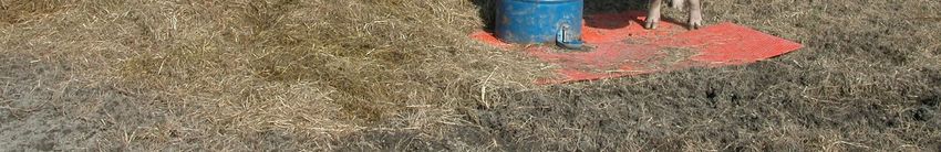
Animals 2020, 10, 1046                                                                               2 of 21

systems to provision niche markets, as observed with the renowned popularity achieved by “Iberico”
products from Spain. This traditional system is found in a unique ecosystem of the Iberian Peninsula
called “La Dehesa”. In the Dehesa, pigs of the ‘Iberico’ heritage breed are managed in a silvopastoral
system where grasses, acorns, chestnuts and other local resources contribute to the origination of the
dry-cured ham [5]. These market trends oriented to products originated in alternative production
systems, should be cultivated to strengthen the consolidation of the pasture-based pork supply chain
and its related niche markets. A market-driven approach could include labelling [6]. In Europe exist
legal certifications that allow the identification of certain attributes in products oriented to specialized
niche markets. Certifications such as IGP (Indication of Geographic Protection) and DOP (Protected
Designation of Origen) indicate that quality traits of the product are linked to the place of production,
processing or preparation, and that specific age-old traditional protocols have been followed [7].
In these niche markets, sustainable practices that integrate elements relevant to the environment,
animal welfare, food safety, and economic viability are drivers for innovation.
      To improve the productivity and animal welfare in pasture pig systems, it is convenient to organize
and manage the herd in functional groups according to their productive stage (breeding, gestation,
farrowing, growers and finishers) [8,9]. Pasture use is an ideal option for managing gestating sows
because older animals can make better use of nutrients from forages, and it provides opportunity
for a wide range of favorable behavorial activities. [10]. Additionally, pasture helps alleviate hunger
in sows fed a restricted diet at maintenance levels [11]. Pregnant sows grazing Lolium perenne and
Trifolium repens pastures, and managed under supplemental feed restriction strategies presented daily
forage intake in the range of 3.4 to 8.2 kg fresh forage + 1.5 kg of supplemental feed, and 6.5 to
8.1 + 3.0 kg of supplemental feed per sow, during spring and summer, respectively [12]. Similarly,
lactating sows grazing the same grass and clover mixture but receiving feed supplement ad libitum
showed lower fresh forage intake (0.2 to 1.6 kg sow−1 d−1 ) [13].
      Reduction of environmental impact is one of the major goals of sustainable livestock production
and imposes underlying pressure to farmers. Indeed, farmers face the challenge of how simultaneously
integrate environmental goals with production system practices oriented to achieve animal welfare,
farm profitability and consumers’ health. Key elements of a successful grazing system include
identifying how many animals to incorporate and defining the grazing period that will minimize the
environmental impact on the resources. Concentrating too many animals could damage the vegetative
ground cover leaving the soil vulnerable to the influence of rainfall, wind and temperature [14].
      Best management practices are designed to support farmers in the search of more sustainable
ways to produce food. But this goal is not easily achieved with grazing pigs which, if left uncontrolled,
could express potentially environmental damaging behavior such as selective grazing, rooting and
the use of preferred dunging areas [15]. Combined with the physical effect of their hooves, swine
natural behavior could deteriorate the ground cover, and increase bare soil, soil compaction, erosion,
and run-off, thus negatively impacting surface and ground water and decreasing pasture production
and productivity [16,17]. Additionally, the grazing of pigs involves a high import of nutrients into
the system through the feed. Grazing animals deposit manure and urine in certain sections of the
paddocks, therefore if the amount of nutrients deposited surpasses the vegetation capacity to use
these nutrients there is a risk of environmental pollution [17]. The amount of nutrients that leave a
pasture system through erosion, runoff and leaching can be reduced by maintaining an appropriate
ground cover, a factor directly linked with the stocking rate and length of access. Indeed, lower ground
cover [18–20] and higher soil structural damage [17,21,22] have been related to increased stocking rate.
      There are many factors to consider when determining suitable stocking rate for swine on
pastures (soil, forage type, weather conditions, animal physiological stage, and management skill) [17].
The effects of stocking rates (ranging from 8 to 92 sows ha−1 ) has been documented [18,19,23–30].
In some European countries, the stocking rates are established based on the projected annual excretion
of N (140 kg N ha−1 ) [30]. To our knowledge, the rotational stocking management system as used in
this work has not been previously evaluated in terms of ground cover maintenance or soil nutrient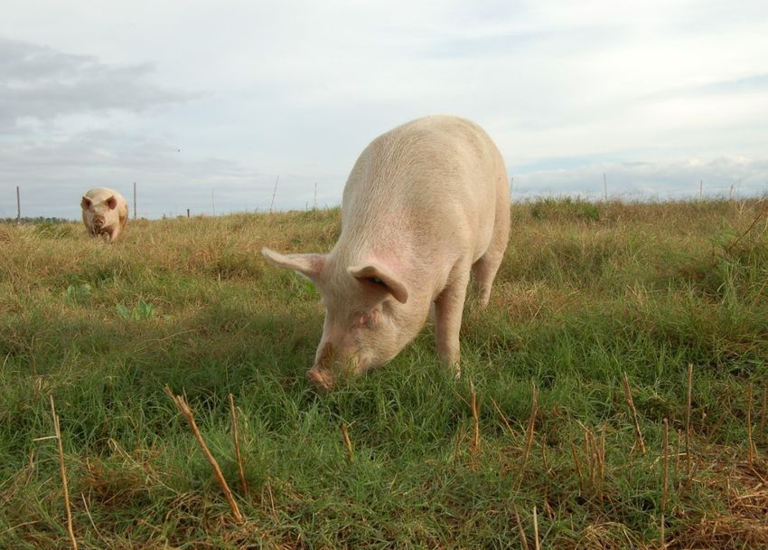
Animals 2020, 10, 1046                                                                            3 of 21

upload. Ground cover maintenance and nutrient management are key elements to reduce the
environmental impact of outdoor swine production [31]. Maintaining a ground cover greater than 75%
and controlling nutrient loading and distribution are considered as best management practices for
pasture pig operations [32]. These best management practices improve soil health and water quality,
by minimizing runoff, soil erosion and water pollution. This study was conducted to evaluate the effect
of three stocking rates (10, 15 or 25 sows-gilts ha−1 ) on ground cover and soil nutrient concentrations
of bermudagrass (Cynodon dactylon L. Pers) paddocks managed in a weekly rotational stocking system.

2. Materials and Methods

2.1. Study Area
     The research was conducted at the Center for Environmental Farming System (CEFS) Field
Research, Education, and Outreach Facility at Cherry Research farm, in Goldsboro (35.38291◦ N,
–78.035846◦ W), North Carolina (USA). The climate is humid subtropical (Trewartha climate
classification), with average temperatures between 10.8 and 22.5 ◦ C and yearly precipitation of
1465 mm. The soils of the experimental site had been classified as Johns sandy loam (Fine-loamy over
sandy or sandy-skeletal, siliceous, semiactive, thermic Aquic Hapludults), and Kenansville loamy
sand (Loamy, siliceous, subactive, thermic Arenic Hapludults), based on US Soil Taxonomy [33]. The
terrain is mostly flat with 0 to 2% slope. The CEFS swine herd is managed in hoop houses using a deep
bedding system. The nucleus of the herd is Yorkshire, and has been kept antibiotic-free for almost
40 years, thus requiring that very strict biosecurity measures must be followed. These biosecurity
measures restricted the availability of animals during the calendar year, thus constraining the timing
of the experiment. The field experiment was conducted over three grazing periods of 8 weeks each
during two consecutive years: January to March of year 1; September to November of year 1; and April
to June of year 2. A 24-week rest period was implemented between each grazing period.

2.2. Animals
     The study was conducted in accordance with the animal use and care guidelines of North Carolina
State University Institutional Animal Care and Use Committee (IACUC 09-021-A). A total of 60 pure
Yorkshire sows and gilts were allotted to one of the three treatments according to pre-experimental
individual live weight to balance live weight across stocking rates. Three different groups of animals
varying in initial live weight (294.2 ± 8.4, 211.9 ± 6.9 and 186.4 ± 3.0 kg for animals used in grazing
period 1, 2 and 3, respectively) and parity were used. Live weight was estimated by weighing the
sows when they were turned in and out of the paddocks. The change in live weight during the graze
periods was equivalent to 1.2 ± 4.36, 5.58 ± 3.03 and 5.51 ± 2.87 kg for animals included in grazing
period 1, 2 and 3, respectively).
     Prior to the experimental period, sows-gilts were kept in straw-bedded hoop barns, but were given
two weeks of acclimation to a wooded outdoor paddock with an electrical fence. At the beginning
of each grazing cycle, animals were arranged in groups of two, three or five corresponding to the
treatments. These groups were randomly assigned to the paddocks where they stayed for the 8-week
grazing cycle.
     During the graze period the animals had free access to shelter and water drinkers located in the
center of the paddock (Figure 1). Shelters were built with repurposed metal grain bins open on one end.
Sows were offered daily in the morning a home-mixed feed containing corn, soybean, minerals and
vitamin mixes. Feed was allocated according to maintenance requirements which averaged 2.0 kg grain
mixture head−1 d−1 plus an additional adjustment of 0.41 kg per every 45 kg of live weight over 180 kg.
During the first grazing period when the environmental temperature declined to 12.8 ◦ C, animals
received an additional 0.20 kg head−1 d−1 per 5.6 ◦ C decline in temperature. Feed was analyzed for
chemical composition by the North Carolina Department of Agriculture and Consumer Services-Farm
Feed Testing Service laboratory. On average, the grain mix contained 161.1 g kg−1 crude protein;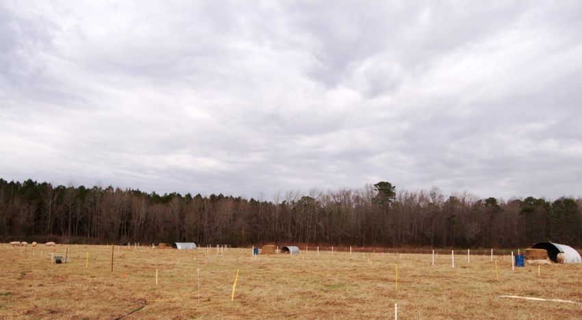
Animals 2020,
Animals 2020, 10,
10, xx 44 of
of 22
22
Animals 2020, 10, 1046 4 of 21
for chemical
for chemical composition
composition by by the
the North
North Carolina
Carolina Department
Department of of Agriculture
Agriculture and and Consumer
Consumer Services
Services
-- Farm
Farm Feed
Feed Testing
Testing Service
Service laboratory.
laboratory. OnOn average,
average, thethe grain
grain mix
mix contained
contained 161.1
−1 crude fat; and 44.5 g kg−1 ash (8.7 g kg−1 Ca; 5.3 g kg−1 P; 2.0 g kg−1 S; 1.7 g kg−1 Mg;
161.1 g g kg
kg−1 crude
−1 crude
43.3 g kg
protein; 43.3
43.3 gg kg
kg-1 crude
-1 crude fat;
fat; and
and 44.5
44.5 g
g kg
kg−1 ash
−1 ash (8.7
(8.7 g
g kg
kg−1 Ca;
−1 Ca; 5.3
5.3 g
g kg
kg−1 P;
−1 P; 2.0
2.0 g
g kg
kg−1 S;
−1 S; 1.7
1.7 g
g kg
kg−1−1 Mg;
protein; −1 Na; 8.4 g kg−1 K; 163 g kg−1 Cu; 281 ppm Fe; 51 ppm Mn; and 139 ppm Zn); net energy
Mg;
1.8
1.8 g
g kg
kg −1 Na; 8.4 g kg −1 K; 163 g kg−1 −1 Cu; 281 ppm Fe; 51 ppm Mn; and 139 ppm Zn); net energy was
1.8 g kg Na; 8.4 g kg K; 163 −1
−1 −1 g kg Cu; 281 ppm Fe; 51 ppm Mn; and 139 ppm Zn); net energy was
was calculated
calculated as 2436
as 2436
2436 kcal
kcal kg
kg kg The
−1 DM. DM.daily
The feed
dailywas
feeddelivered
was delivered
once dayonce
day day−1
−1 onto onto
mats matsfrom
made made from
rubber
calculated as kcal −1 DM. The daily feed was delivered once −1 onto mats made from rubber
rubber used
used conveyor conveyor
conveyor belts belts
belts providing providing
providing space space
space enough
enough toenough
to allow to allow simultaneous
allow simultaneous
simultaneous access
access to access
to feed to feed
feed (each (each
(each sow
sow had
hadsow
used 11
had 1
lineal lineal
m of m
the of
matthe mat available,
available, Figure Figure
2). 2).
lineal m of the mat available, Figure 2).
Figure 1.
Figure 1. The
The service
service areas
areas with
areas withthe
with theshelter
the shelterand
shelter andaaawater
and waterbarrel
water barrelfunctioning
barrel functioning
functioning as
asas aa drinker
drinker
a drinker were
were
were located
located
located in
in
in the
thethe center
center
center of
of of the
thethe paddocks.
paddocks.
paddocks. AA A PVC-coated
PVC-coated
PVC-coated metal
metal
metal slat
slat
slat waswas
was placed
placed
placed under
under
under the
thethe barrel
barrel
barrel to
to to reduce
reduce
reduce damage
damage
damage to
to the
the
to the soil
soilsoil structure.
structure.
structure. (January
(January
(January to March,
to to March,
March, year
year 1).
1). 1).
year
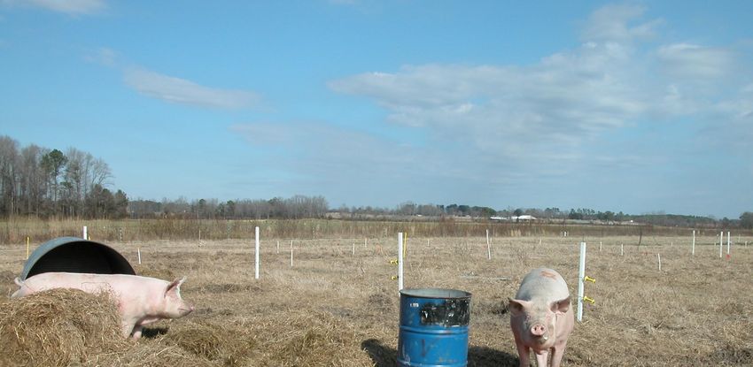
Figure 2.
Figure
Figure 2. Mats
2. Mats from
Mats from
from aaa repurposed
repurposed rubber
repurposed rubber conveyor
rubber conveyor belt
conveyor belt were
belt were used daily
were used
used daily to
daily to offer
to offer aaa farm-made
offer farm-made grain
farm-made grain
grain
mixture.
mixture. (January
mixture. (January to
(January to March,
to March, year
March, year 1).
year 1). The
1). The snow
The snow is
snow is not
is not frequent
not frequent in
frequent in the
in the area
the area and
area and only
and only lasted few
lasted few
only lasted days.
few days.
days.
2.3. Pasture
2.3. Pasture Management
Management
A 1.25-ha
A 1.25-hapasture
1.25-ha pastureestablished
pasture establishedwith
established Coastal
with
with bermudagrass
Coastal
Coastal waswas
bermudagrass
bermudagrass divided
was into into
divided
divided two blocks,
into whichwhich
two blocks,
two blocks, were
which
further
were divided
were further
further into three
divided
divided intorectangular
into three paddockspaddocks
three rectangular
rectangular each. Theeach.
paddocks paddocks
each. The differed
The paddocks
paddocks slightly in dimensions
differed
differed slightly in
slightly in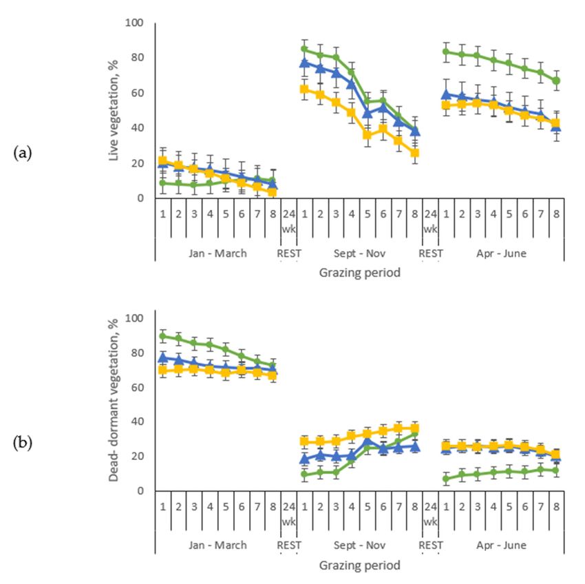
Animals 2020, 10, 1046 5 of 21
Animals
Animals2020,
2020,10,
10,xx 55of
of22
22
dimensions
among among
the two
dimensions the
blocks
among two
twomblocks
(59.4
the × 34 m(59.4
blocks mm××m
vs. 66.0
(59.4 34
34×m vs.
m30.6 66.0
vs.m, m
for
66.0 ××30.6
mblock
30.61 m,
m,for
and 2, block
for block11and
and2,
respectively), respectively),
2,and measured
respectively),
and 2 . Each paddock
an measured
average an
2019.6 maverage 2019.6 m
and measured an average 2019.6 m . Each paddock was divided using plastic step-posts and
22. Each
was paddock
divided using was divided
plastic using
step-posts andplastic step-posts
electrified poly-wire
and
electrified
fencing poly-wire
into
electrified fencing
fencing into
nine equal-sized
poly-wire into nine
sections equal-sized
nine(Figure sections
3; Figure
equal-sized 4). (Figure
sections (Figure3; 3; Figure
Figure4).
4).
Figure 3.
3. Experimental
Figure3. Experimental setup.
Experimental setup. Paddock
setup. Paddock dimensions
dimensionsin
dimensions in the
the field’s
field’s replicates
replicates were
were slightly
slightly different.
different.
(Replicate 1: 30.6 m ×
×
(Replicate 1: 30.6 m × 66.0
66.0 m
m and
and Replicate
Replicate 2:
2:
Replicate 2: 34.0
34.0 m
m ×
× 59.4
59.4 m).
m). The
The figure
figureis
isnot
notdrawn
drawn to
to
× 59.4 m). The figure is not drawn to scale. scale.
scale.
Figure 4.
4.View
Figure4.
Figure Viewof
View ofone
of onefield
one fieldreplicate
field with
replicatewith
replicate three
withthree paddocks.
paddocks.The
threepaddocks. Theservice
The serviceareas
service areascan
areas canbe
can beidentified
be with
identifiedwith
identified the
withthe
the
shelters, the
shelters,the
shelters, barrel-drinkers,
thebarrel-drinkers, and
barrel-drinkers,and piles
andpiles of
pilesof hay.
ofhay. At
hay.At the
Atthe far
thefar left,
farleft, four
left,four sows
foursows in
sowsin a graze
inaagraze subplot.
grazesubplot. (January
subplot.(January
(Januarytoto
to
March, year
March,year
March, 1).
year1).
1).
The 2
The central
central section
section (representing
(representing 11.1%11.1% ofofthethepaddock,
the paddock,224.4
paddock, 224.4m
224.4 m22)) was
m was considered
considered thethe service
service
section drinkers
drinkers were located.
located. The
section where shelters and water drinkers were located. The other eight sections were managed as
where shelters and water other eight sections were managed as
graze
grazesections
sectionsresulting
resultingininan
aneight
eightsubplot rotation
subplotrotation (Figure
rotation(Figure
(Figure5). 5).
5).Animals
Animalshad hadpermanent
permanentaccess
accessto tothe
the
service
service sections,
servicesections,
sections,andand simultaneously
andsimultaneously
simultaneously totoone
to one of
of the
of the
one grazing
grazing
the grazing sections
sections on aon
sections aa weekly
weekly
on basis.basis.
weekly Each Each
basis. of theof
Each of the
graze
the
graze
grazesections
sections sections was
was grazed
was grazed once (7
grazed once
d of
once (7 ddofof occupation)
(7occupation) per
per grazing
per grazing
occupation) period.
period.
grazing In
In the
period. Inthethegraze
graze section
section
graze currently
currently
section currentlyin
in
in use,
use, the the
use, the feed
feed was was
feed was provided
provided over
over used
provided used
used conveyor
overconveyor belts
belts acting
conveyor beltsasacting as
as feeders.
feeders.
acting The location
feeders. The location
The of of
of these
these “feeders”
location these
“feeders”
changed
“feeders” changed
daily within
changed daily within
within the
the respective
daily respective
thesection. Thesection.
respective water was
section. The
The water
water was
supplied using
was supplied using
metal barrels
supplied metal
usingwith
metal barrels
attached
barrels
with
with attached
water-cup
attached water-cup
drinkers.
water-cup drinkers.
A PVC-coated
drinkers. AA PVC-coated
metal perforated slat
PVC-coated metal
metal (61 perforated
cm × 122 cm,
perforated slat (61
3/8”
slat cm
cm ×× 122
openings)
(61 was
122 cm, 3/8”
placed
cm, 3/8”
openings)
openings)was wasplaced
placedunder
undereach
eachdrinker.
drinker.The Thestocking
stockingdensity
densitywaswasequivalent
equivalentto to10,
10,1515and
and25 25sows-
sows-
gilts
gilts ha
ha−1−1 (224.4,
(224.4, 149.6
149.6 and
and 89.8
89.8 m m22 sow-gilt
sow-gilt−1−1 week
week−1−1,, respectively;
respectively; Table
Table 1). 1). The
The paddocks
paddocks werewere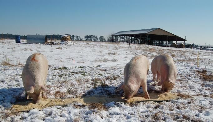
Animals 2020, 10, 1046 6 of 21
Animals 2020, 10, x 6 of 22
under each drinker. The stocking density was equivalent to 10, 15 and 25 sows-gilts ha−1 (224.4, 149.6
and 89.8 m 2 sow-gilt−1 week−1 , respectively; Table 1). The paddocks were managed with the same
managed with the same stocking rate treatments during the three grazing periods. Temporary electric
stocking rateused
fencing was treatments during
to control accessthe
to three grazing periods.
the designated Temporary
sub-section electric
each week. Each fencing was used to
of the 8 sub-sections
control
was grazed for 7 days of the 56-day grazed period. Grazing periods were calendar-fixed grazed
access to the designated sub-section each week. Each of the 8 sub-sections was for
with a 24-
7week
daysrest
of the 56-day grazed period. Grazing periods were calendar-fixed with a 24-week rest
period among consecutive grazing periods. No fertilizer was applied during the course of period
among consecutive grazing periods. No fertilizer was applied during the course of the experiment.
the experiment.
Figure
Figure 5.
5. Gilts
Gilts in
in aa graze
graze section
section (September
(September to
to November, year 1).
November, year 1).
Table 1. Stocking
Table 1. Stocking rates
rates for sows-gilts grazing
for sows-gilts grazing bermudagrass
bermudagrass for
for three
three grazing
grazing cycles
cycles of
of eight weeks in
eight weeks in
an 18-month period.
an 18-month period.
Grazing
Grazing Cycle
Cycle Stocking
Stocking Rate, Rate, ha−1ha−1
Sows-Gilts
Sows-Gilts
10 10 15 15 25 25
m head m2 head−1
2 −1 1000 1000 667 667 400400
1st,1st,
JanJanuary
to March Kg Live weight
to March Kg Liveha−1
weight ha−12942 2942 4413 4413 7355 7355
2nd, September to November −1 2119 3179 5298
2nd, Sept to Nov Kg Live weight haKg Live weight
−1 ha 2119 3179 5298
3rd, April to June Kg Live weight ha−1 1864 2796 4660
3rd, Apr to June Kg Live weight ha −1 1864 2796 4660
2.4. Ground Cover Estimation
Ground cover
cover estimation
estimationwaswasconducted
conducted weekly
weekly using
using a modified
a modified stepstep point
point method
method [34]. [34].
The
The ground
ground cover
cover waswas differentiated
differentiated into
into three
three components:live
components: livevegetation
vegetation(including
(includinggrasses,
grasses, forbs,
forbs,
leaves and stems), dead-dormant vegetation (litter-plant residues, standing dormant and senesced or
dead vegetation) and bare soil. To To assess ground cover, each paddock was marked with 24 equally
spaced transects using pieces of PVC pipes (70 cm long by 1.27 cm diameter). Every other step along
the transect
transect represented
representedaasampling
samplingpoint,
point,inin each
each of of which
which thethe ground
ground cover
cover waswas characterized
characterized and
recorded.
and On average,
recorded. 28 sampling
On average, pointspoints
28 sampling were recorded per transect
were recorded providing
per transect 672 points
providing 672 within
points
each treatment
within paddock.
each treatment GroundGround
paddock. cover was calculated
cover with thewith
was calculated following equation:
the following GroundGround
equation: cover =
cover = live vegetation
live vegetation + dead-dormant
+ dead-dormant vegetation vegetation
[34]. Ground cover
[34]. was determined
Ground cover wasweekly, but only
determined data
weekly,
corresponding
but to the last week
only data corresponding (8th
to the week)
last weekof(8th
each grazing
week) period
of each were
grazing included
period wereinincluded
the statistical
in the
analysis. analysis.
statistical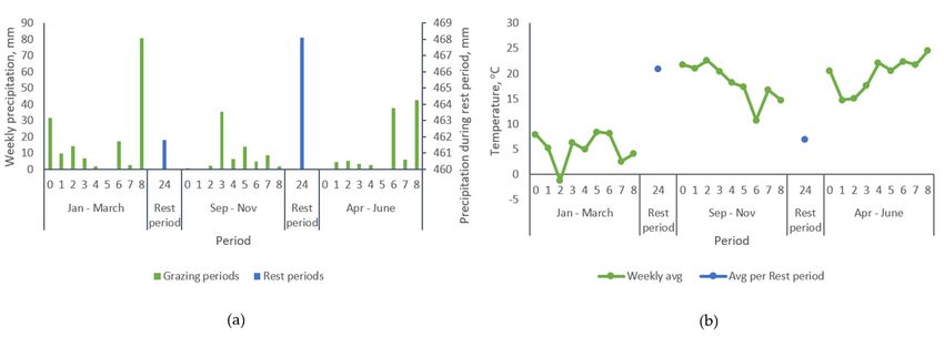
Animals 2020, 10, 1046                                                                                7 of 21

2.5. Soil Samples
      Soil samples were collected and assembled before starting the experiment, and following the
removal of the animals from the paddocks after the first and third grazing periods. Paddock portions
showing evidence of feed waste and manure deposits at the soil surface were excluded in the sampling
process. The initial sampling was conducted using a hand probe (2-cm diameter) to a sampling depth
of 30 cm. Five soil cores were taken from each of the nine sections of the paddocks, combined (45 cores)
and mixed to form one composite sample per paddock (n = 6). One week after the animals were
removed at the end of the first grazing period, soil samples were collected using a hand probe to two
depths: 0 to 15 and 15 to 30 cm. Each sample was made up of 15 soil cores randomly gathered from
each paddock section. Those samples were later combined and mixed per depth to yield a sample
corresponding to the service section, and a sample for the graze section (this last one, containing 20 cc
subsamples from each of the eight grazing sections). A total of 24 samples were sent to the laboratory.
Following the third grazing period (nine days after animal removal) one core soil sample was taken
from the center of each of the nine sections of the paddock using a soil coring device (3.2 cm diameter)
installed on a truck (Model GSRPS Giddings Machine Company, Windsor, CO). These samples were
collected to four sampling depths (0 to 15, 15 to 30, 30 to 60 and 60 to 90 cm) resulting in 216 samples.
      Soil samples were air-dried at room temperature, gently crushed, sieved through a 2-mm mesh [35]
and sent to the North Carolina Department of Agriculture and Consumer Services Agronomic Division,
Soil Testing Section laboratory for standard analysis using Mehlich-3 extraction methodology (Mehlich
buffer acidity) for Ca, P, K, Mg, Na, S, Cu, Mn, Zn, and Fe. Samples were also analyzed for
ammonium (NH4 + ) and nitrate (NO3 - ) concentrations (1 M KCl soil extracts analyzed on a Quick Chem
8000 LACHAT) [35] at North Carolina State University Environmental and Agricultural Testing Service
laboratory. The amount of nutrients imported to the system through animal feed were estimated.

2.6. Experimental Design and Statistical Analysis
      A randomized complete block design with a split–split plot arrangement of treatments was used
to analyze ground cover data, while soil data were evaluated employing a split plot complete block
design with a factorial treatment arrangement. For ground cover, the main plot factor was the grazing
period (January to March, year 1, September to November, year 1 and April to June, year 2), stocking
rate (10, 15 and 25 sows-gilts ha−1 ) was the subplot factor and section of the paddock (grazing and
service sections) represented the sub-subplot factor. Two independent analyses were conducted for the
soil samples collected after the first and the last (third) group of sows. For soil nutrients, stocking rate
was considered as the main plot factor and soil sampling depth (0 to 15 and 15 to 30 cm; or 0 to 15; 15 to
30; 30 to 60 and 60 to 90 cm, for the sampling conducted after the first or after the third grazing period,
respectively) as the subplot factor. Treatments were randomly assigned to the paddocks and each
paddock was considered as the experimental unit. All treatments had two field replicates (blocks).
      Statistical data analyses were performed with the software SAS version 9.4 (SAS Institute Inc.,
Cary, NC, USA) using the PROC GLIMMIX (generalized linear mixed models) [36]. In the models
for ground cover, grazing period, stocking rate, section of the paddock and their interactions were
treated as fixed effects. Blocks and its interactions with grazing period, stocking rate and section of the
paddock were considered random effects. In the models for soil nutrients, block and its interactions
with stocking rate and sampling depth were included as random effects and stocking rate, sampling
depth and their interaction as fixed effects. Differences were considered significant when p ≤ 0.05,
and p ≤ 0.10 were noted as a tendency. Mean separation was conducted using least-squares means
including the ADJUST and SIMULATE options.

3. Results
     The cumulative precipitation and average daily temperature recorded during the experiment are
presented in Figure 6. The precipitation was 164.2, 73.5 and 101.70 mm for grazing cycles 1, 2 and 3,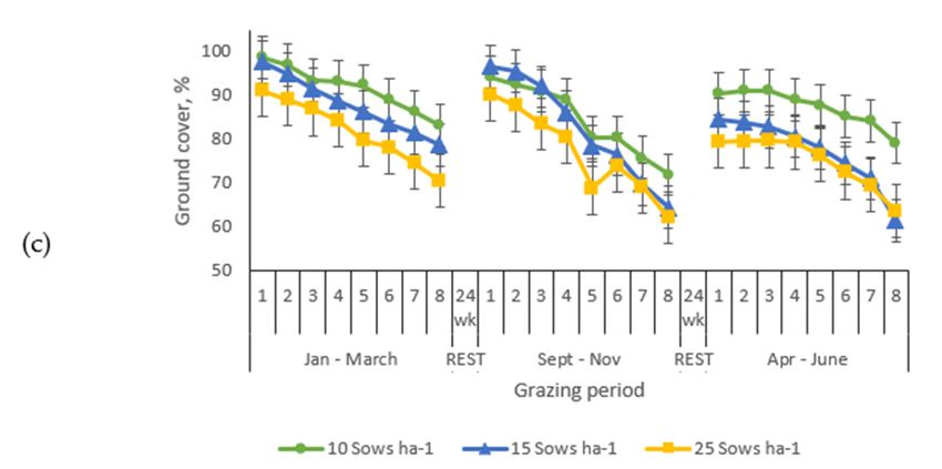
Animals 2020, 10, x                                                                                            8 of 22

3. Results
Animals 2020, 10, 1046                                                                                         8 of 21
       The cumulative precipitation and average daily temperature recorded during the experiment
 are presented in Figure 6. The precipitation was 164.2, 73.5 and 101.70 mm for grazing cycles 1, 2 and
 3, respectively.
respectively.       Similarly,
                Similarly, the the  average
                                average       daily
                                          daily      temperature
                                                temperature          for same
                                                                for the  the same    periods
                                                                               periods    werewere
                                                                                                5.16, 5.16, 18.2 19.9
                                                                                                       18.2 and   and
◦19.9
  C. In°C. In addition,
        addition,        the amount
                   the amount          of precipitation
                                 of precipitation         registered
                                                   registered   during during   theand
                                                                         the first  firstsecond
                                                                                          and second    rest periods
                                                                                                 rest periods    were
 were 461.80
461.80  mm and mm468.10
                     and 468.10  mm, respectively,
                          mm, respectively,    and theand   the temperature
                                                        temperature     variedvaried    from
                                                                                from 21.0      7.0 ◦to
                                                                                            to21.0   C 7.0 °C during
                                                                                                       during   those
 thoseintervals.
time    time intervals.   Accordingly,
                  Accordingly,           the weather
                                  the weather            conditions
                                                conditions    during during    the experimental
                                                                       the experimental              period
                                                                                            period did    not did
                                                                                                              havenota
 have a negative
negative    impact impact   on bermudagrass
                     on bermudagrass     growthgrowth      and survival.
                                                  and survival.            Soil disturbance,
                                                                    Soil disturbance,           vegetation
                                                                                          vegetation   damagedamage
                                                                                                                  and
 and leaching
leaching         of nutrients
           of nutrients  can becan  be highly
                                highly  relatedrelated
                                                 to soilto soil moisture
                                                         moisture           conditions.
                                                                    conditions.           Only during
                                                                                   Only during            weekofeight
                                                                                                 week eight        the
 of the
first   firstperiod
      graze   graze period
                      was thewas  the rainfall
                              rainfall         sufficient
                                       sufficient to havetopotentially
                                                              have potentially
                                                                          impactedimpacted    those parameters.
                                                                                     those parameters.

     Figure 6. Cumulative precipitation (a) and average temperature (b) registered during the experimental
      Figure 6. Cumulative precipitation (a) and average temperature (b) registered during the
     period. Source: CHRONOS database - State Climate Office Of North Carolina [37] and own estimation.
      experimental period. Source: CHRONOS database - State Climate Office Of North Carolina [37] and
      own estimation.
3.1. Ground  Cover
      This study
 3.1. Ground       monitored ground cover changes over time in graze and service areas of the paddocks.
               Cover
Ground cover in the graze sections of the paddocks generally declined weekly throughout each of the
grazingThis  study
          cycles,    monitored
                  following      ground
                             a similar    coverforchanges
                                       pattern              over time
                                                   all the periods       in graze
                                                                     (Figure 7).   and service areas of the
 paddocks.
      During the first two grazing cycles, the ground cover within the graze sectionsweekly
              Ground   cover in the graze sections  of the paddocks    generally declined        throughout
                                                                                           was similar for all
 each  of the grazing  cycles, following  a similar pattern  for all the periods (Figure 7).
stocking rates. However, in the third period, there was less cover in paddocks managed with 15 or 25,
compared to those managed with 10 sow ha−1 . The mean ground cover values during the experimental
period were greater than 65%, even for the paddocks managed with the higher stocking rate. The rest
period (168 days) between grazing cycles allowed the ground cover to recover in all the paddocks,
reaching 93.8 and 85% at the beginning of the second and third period, respectively.
      At the end of each grazing period the ground cover (in both graze and service areas) was affected
by the grazing cycle (p = 0.0011), the stocking rate (p = 0.0423), the paddock section (graze or service)
(p < 0.0001) and the interaction of grazing cycle x paddock section (p = 0.0514) (Table 2, Figure 8).
Ground cover was 72.6% at the end of the first grazed cycle, but only 48.3% at the end of the 2nd and 3rd
graze cycles (47.1 and 49.6%, respectively). Paddocks managed with 10 sows-gilts ha−1 had significantly
more (35.4 %) ground cover than paddocks with 25 sows-gilts ha−1 (Table 2). However, there were no
significant differences in ground cover between the stocking rates 10 and 15 sows-gilts ha−1 (average
60.7%). The cover was similar also for 15 and 25 sows-gilts ha−1 (average 52.1%). The graze section of
the paddocks had 68% more ground cover than the service sections (Table 2) except at the end of the
first grazing period, when no differences in ground cover were detected among both sections of the
paddocks which averaged 72.8% (Table 2; Figure 8). The interactions grazing cycle x stocking rate,
stocking rate x paddock’s section, and grazing cycle x stocking rate x paddock’s section were found to
be not statistically significant (p > 0.05).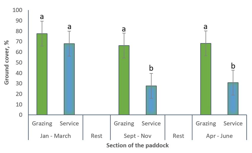
Animals 2020, 10, 1046                                                                                                               9 of 21
      Animals 2020, 10, x                                                                                                      9 of 22

             Animals 2020, 10, x                                                                                    10 of 22

             there were no significant differences in ground cover between the stocking rates 10 and 15 sows-gilts
             ha−1 (average 60.7%). The cover was similar also for 15 and 25 sows-gilts ha−1 (average 52.1%). The
             graze section of the paddocks had 68% more ground cover than the service sections (Table 2) except
             at the end of the first grazing period, when no differences in ground cover were detected among both
             sections of the paddocks which averaged 72.8% (Table 2; Figure 8). The interactions grazing cycle x
             stocking rate, stocking rate x paddock’s section, and grazing cycle x stocking rate x paddock’s section
             were found to be not statistically significant (p > 0.05).

                   Table 2. Final vegetative ground cover (%, means and standard error) estimated after animal removal
                   in bermudagrass paddocks managed with sows-gilts during three grazing periods.

                                                                       Vegetation (%)
                                          Factors
                                                          Living    Dead-Dormant Ground Cover
                                   Grazing period
                                   p
Animals 2020, 10, 1046 10 of 21
Table 2. Final vegetative ground cover (%, means and standard error) estimated after animal removal
in bermudagrass paddocks managed with sows-gilts during three grazing periods.
Vegetation (%)
Factors
Living Dead-Dormant Ground Cover
Grazing period
pAnimals 2020, 10, 1046 11 of 21
Table 3. Soil nutrients (mg kg−1 ) in bermudagrass paddocks following the first eight weeks of grazing with sows-gilts (January to March).
Factors NH4 + NO3 − P K Ca Mg S Mn Zn Cu Na Fe
(mg kg−1 )
Initial values 8.5 2.4 470.6 193.7 863.8 182.2 17.8 17.1 9.6 1.0 16.8 1081.2
SE ± 1.1 ± 0.5 ± 76.6 ± 24.9 ± 75.4 ± 18.9 ± 1.1 ± 4.6 ± 3.2 ± 0.2 ± 0.8 ± 108.9
Stocking rate
p 0.5845 0.4513 0.6888 0.3215 0.5459 0.3984 0.3218 0.4859 0.3426 0.2753 0.4162 0.2570
10 Sows ha−1 8.5 3.2 419.4 176.3 779.1 162.0 18.3 15.2 6.5 0.8 20.3 1099.0
15 Sows ha−1 12.7 5.3 488.3 195.9 888.5 181.8 19.6 18.2 11.6 1.2 25.0 1027.6
25 Sows ha−1 10.9 5.3 492.4 213.0 851.6 187.5 21.4 18.0 8.2 1.0 25.4 1335.0
SE ± 2.7 ± 1.2 ± 171.4 ± 25.5 ± 64.5 ± 11.9 ± 1.2 ± 10.4 ± 4.9 ± 0.24 ± 2.5 ± 10.8
Soil depth
p 0.0843 0.0110 0.6632Animals 2020, 10, 1046 12 of 21
Table 4. Soil nutrients (mg kg−1 , means and standard error) in bermudagrass paddocks following three eight-week periods of grazing with sows-gilts (January to
March, year 1; September to November, year 1; April to June, year 2).
Factors NH4 + NO3 − P K Ca Mg S Mn Zn Cu Na Fe
(mg kg−1 )
Initial values 8.5 2.4 470.6 193.7 863.8 182.2 17.8 17.1 9.6 1.0 16.8 1081.2
SE ± 1.1 ± 0.5 ± 76.6 ± 24.9 ± 75.4 ± 18.9 ± 1.1 ± 4.6 ± 3.2 ± 0.2 ± 0.8 ± 108.9
Stocking Rate
p 0.0082 0.0177 0.0002 0.0544 0.1156 0.6400 0.2184 0.6795 0.0001 0.0017 0.649 0.1167
10 Sows ha−1 9.0 b 0.7 b 280.6 b 135.9 b 633.0 144.8 14.9 12.6 5.1 b 0.7 b 13.7 1020.3
15 Sows ha−1 12.1 a 0.8 b 346.1 b 184.0 a 605.6 138.5 18.5 13.6 5.5 b 0.8 b 14.8 1185.2
25 Sows ha−1 13.2 a 1.6 a 428.9 a 162.9 a,b 677.6 147.7 16.7 13.3 9.4 a 0.9 a 14.2 1163.0
SE ± 1.3 ± 0.4 ± 172.9 ± 23.3 ± 51.5 ± 29.7 ± 2.5 ± 9.6 ± 3.4 ± 0.2 ± 1.1 ± 58.2
Soil depth
p 0.0002 0.9014Animals 2020, 10, 1046 13 of 21
3.3. Estimated Excretion of Nutrients into the System
The estimated amount of N and P imported to the system from the feed over the course of
the three grazing cycles are presented in Table 5. The estimated N inputs ranged from 113 kg ha−1
(10 sows-gilts ha−1 ) to 280 kg ha−1 (25 sows-gilts ha−1 ). Phosphorus input ranged from 23 to 58 kgs
ha−1 for the 10 to 25 sows-gilts ha−1 , respectively.
Table 5. Estimated Total N and Total P (kg ha−1 ) imported to the system via feed offer.
Grazing Cycle
Stocking Rate
1st 2nd 3rd Total
sows-gilts ha−1 Nitrogen, kg ha−1
10 50 33 30 113
15 75 49 45 169
25 124 82 74 280
sows-gilts ha−1 Phosphorus, kg ha−1
10 10 7 6 23
15 15 10 9 34
25 26 17 15 58
4. Discussion
The adoption of the appropriate stocking rate for a pasture system is a critical management decision
because it influences animal performance, long-term farm productivity, economic outcomes, wildlife
and natural resources. The impact by grazing animals is the result of diverse interrelated comportments
including defoliation, treading, trampling, and manure deposition [38]. The implementation of high
stocking rates could magnify the undesirable impacts of grazing animals [38]. Previous research has
shown the importance of implementing a suitable stocking rate to limit the extent of the damage that
grazing pigs could exert to the vegetation and the soil [18,39,40]. The eight-week rotation scheme
as evaluated fits in systems where sows-gilts are group-managed in breeding paddocks and moved
to gestation paddocks after the second gestation control conducted after the fifth week following
mating (38–42d) [41], or in farrowing–lactating paddocks where sows are moved in one week before
the farrowing date and removed after weaning [31].
4.1. Ground Cover
Maintaining ground cover in outdoor pig systems is critical to controlling water, soil and nutrient
movement off site. In these production systems service areas (feeding, watering, housing) receive the
greater impact of the pigs. Therefore, it is necessary to manage the paddock in such a way that those
service areas can be buffered by grassed areas to minimize runoff and erosion. The morphological
and physiological traits of bermudagrass, a warm season perennial species adapted to different types
of soils and climates, that shows aggressive growth, good grazing tolerance, and ability to produce
biomass of good quality forage when soil nutrients are not limiting [42], make this grass suitable for this
kind of systems. Its growth habit and reproductive mechanisms (rhizomes, stolons, and extensive root
mass) allowed it to endure the grazing, rooting, trampling and lounging behaviour of the sows, and to
recover during the rest periods between successive grazings. The final ground cover reported after the
three grazing periods (72.6, 47.1 and 49.6% for the first, second and third grazing periods, respectively)
demonstrates the potential of bermudagrass inclusion in pasture-based pig systems. The final ground
cover, however, was lower than the 75% recommended to minimize runoff and erosion [32,43]. The first
period (January to March) coincided with winter months when bermudagrass is dormant. During
that season, most of the ground cover consisted of dead-dormant vegetation (69.1%, Figure 7) which
was not nutritionally valuable nor palatable, thus limiting sows foraging behavior and their impact
on the vegetation. Besides, pigs tend to decrease their activity during the coldest days of winter asAnimals 2020, 10, 1046 14 of 21
a saving-energy strategy [44]. Additionally, the rooting behavior could have been restricted by soil
hardness [45–47]. Dormant winter rhizomatous and stoloniferous vegetation (bermudagrass) appears
to provide suitable ground cover, even in service areas where animals lounged and drank for eight
consecutive weeks. Conversely, the second (September to November) and third (April to June) grazing
periods corresponded to fall and spring when the live vegetation accounted on average for 25.8% of
the ground cover at the end of each cycle. This fact could have elicited the foraging behavior of the
sows attracted by the live vegetation. Softer soil conditions, as a consequence of rainfall, could have
made rooting easier [48–50]. Additionally, warmer temperatures could have triggered more rooting for
thermoregulation purposes, increasing paddock surface damage [51]. Moreover, it has been noticed
that pigs tend to impact already affected areas and enlarge existing bare soil spots. What have been
called “grazed patches perpetuating”, showing the lack of random area utilization [52]. Conversely, a
greater amount of grass cover during summer than during winter (80 vs. 50%) has been reported in
paddocks managed with stocking rate of 32 sows ha−1 indicating the existence of a seasonal pattern [53],
and highlighting the effect of local (soil, forage, management) and climatic conditions.
Some authors [54] suggest expressing stocking rates in terms of kg of live weight ha−1 instead of
the number of animals ha−1 when analyzing the impacts of grazing animals on the grassland ecosystem.
In the current study, the heavier animals were used in the first grazing cycle (38% and 58% heavier than
animals in the second and third grazing cycle, respectively), during winter months and showed the
greater final ground cover (72.6 vs. 48.3%). In spite of each grazing period corresponded to different
season, there was no significant interaction between grazing cycle and stocking rate for ground cover,
which decreased from 65.0 to 48.0% for the lowest and the highest stocking rates, respectively. Similar
results have been reported for different forages species [18,48,55,56].
In the study herein, differences in ground cover were detected among the sections of the paddocks,
with graze areas showing 68% more ground cover than the service sections, which represented 11.1%
(1/9) of the paddock area. The lower ground cover of the service sections could represent higher risks
for runoff and nutrient leaching. The greater impact on the ground cover observed in the service
sections is attributed to the permanent access of sows to this area of the paddocks where drinkers
and shelters were located. Conversely, the access to one of the eight graze and feeding sections was
sequential, and allocated on a weekly basis determined by the rotation. The grazing sections were
occupied only one week during each grazing cycle. It has been previously reported that sows show a
tendency to concentrate their activities to the areas adjacent to shelters and huts [39,57]. Estimated
weighted averages showed an overall ground cover of 67.5% for the paddocks under evaluation across
both sections (service and graze areas) and the three grazing cycles. Similarly, weighted average of
final ground cover considering both sections of the paddocks showed that only paddock managed
with 10 sows-gilts ha−1 were able to reach the 75% ground cover conservation goal (75.3, 65.8 and
61.6% final ground cover for 10, 15 and 25 sows-gilts ha−1 , respectively). To maintain 75% cover on the
entire paddock would require an average of 79% ground cover on the 8 graze sections. The rotational
system tested in this experiment located the service area in the center of the paddock surrounded by
the grazing paddocks, thus minimizing potential runoff that could escape from the service section
(Figure 3).
4.2. Soil Nutrient
It could be expected that pastures with a greater number of grazing animals would show an
increased probability for manure deposition and in consequence greater soil nutrient loads [58].
The sows grazing in the first grazing cycle (January to March) received a greater allocation of feed.
They were bigger than the animals used in the two other grazing cycles, but also were supplied
additional feed for thermoregulation to compensate for lower environmental temperatures. However,
no differences in nutrient content among soil samples from paddocks managed with different stocking
rate was noticed in the soil samples collected after removal of the first group of grazing sows. Differences
were only observed among samples collected at different depths showing greater accumulation ofAnimals 2020, 10, 1046 15 of 21
nutrients in the upper soil layer, except for NH4 + ; P and Na, which did not present differences along
the soil profile. Conversely, Fe values were 13% higher in the bottom (15 to 30 cm) layer (Table 3).
The paddocks responded similarly to management with different stocking rates and did not show
a significant impact of stocking rates on soil nutrients concentrations. The differences in amount of
feed and consequently in excretion may have been balanced by bermudagrass uptake [18]. The lack
of a more marked effect of stocking rates could also be attributed to the rotational stocking system
implemented, which allowed the grass a rest period to recover after one week of grazing, and may have
led to better nutrients distribution and utilization [59]. Similarly, it may also be possible that the time
lapse between manure deposition during the grazing period and the soil sampling date was not long
enough to allow the mineralization of organic matter to take place. As the first grazing period was in
winter time, the natural decomposition processes could have been delayed [60]. Similarly, an increase
in extractable phosphorus in soils managed with lactating sows for six months it has been reported,
P levels kept rising even after animal removal [39].
In contrast, the samples collected in the study herein after the third grazing period differed in soil
nutrient concentrations according to stocking rates (Table 4). Paddocks managed with 25 sows-gilts
ha−1 , showed greater soil concentrations of NH4 + ; NO3 - , P; Zn and Cu (46.7, 128.6, 52.9, 84.3 and 28.6%
more, respectively) than paddocks managed with 10 sows-gilts ha−1 . As these nutrients are major
components of pig manure, it may be assumed that the variation of these nutrients detected among the
paddocks could be reflecting additional manure deposited in the paddocks that were more intensively
managed. Paddocks managed with the higher stocking rates received more nutrients to the system via
animal feed and mineralization of the soil organic matter [58]. The presence of greater (35%) ground
cover in paddocks managed with the lower stocking rate (10 sows-gilts ha−1 ) could have partially
contributed to the reduction in the soil nutrient levels as a consequence of plant uptake [19].
Similarly to the findings of the previous set of samples, the nutrient concentrations varied also
according to sampling depth (Table 4) with greater concentrations of NH4 + , P, K, Ca, Mg, S, Mn, Zn
and Cu in samples collected from the upper soil strata (0 to 15 cm). The amount of P and K did not vary
in the first (0 to 15 cm) and second (15 to 30 cm) layers of soil but showed higher values than in deeper
soil strata. However the soil P concentrations in the 30 to 60 and 60 to 90 cm layers (315.7 and 161.6 mg
kg−1 , respectively) are high enough [61] to be considered as evidence of movement through the profile.
The relatively low input of P over the course of the three graze cycles resulted in no differences in soil
P between the first two layers of soil. While being grazed, the additional organic matter deposited on
the soil surface will eventually decay and release its components in the soil profile, circumstance that
could increase the concentration of nutrients in the soil upper layer. The differences among nutrients
along the soil layers could be indicating what portions of these nutrients may have moved deeper into
the soil profile. Irregular dispersion of soil P concentrations in different areas of paddocks managed
with pigs have been previously reported, with greater concentrations of P at the deeper soil layers
around feeders, huts and wallows [62]. The results obtained herein are in agreement with previous
studies where it was indicated an influence of the stocking rates and soil sampling depth on soil nitrate
concentrations [20,60,63].
Perennial forages have been included in nutrient management programs to manage soils fertilized
with swine manure. In the southeast of the USA, different cultivars of bermudagrass have shown good
potential for this purpose. However, differences in the nitrogen use efficiency among cultivars have
been found [42]. Previous studies have shown annual uptake values for this species in the range of
314 to 382, and 44 kg ha−1 yr−1 of N and P, respectively. The species has also shown potential for the
extraction of Ca, K, Mg, Cu, Fe, Mn, and Zn [64]. Although excessive or prolonged application of
manure could cause nutrients accumulation in the soil, with increased environmental risks.
In this study, a simplified N and P balance was conducted, under the assumption that the inputs
to the systems were represented by the feed offered to the animals and entering the system by nutrients
deposition via sow excreta. Similarly, little nutrients were expected to leave the system because no
major changes were observed in animal weight, and there was no removal of bermudadgrass biomassAnimals 2020, 10, 1046 16 of 21
from the paddocks. Under these conditions, it could be expected a surplus of N close to the values of
the imported N. The estimated N inputs ranged from 113 kg ha−1 to 280 kg ha−1 , while P input varied
from 23 to 58 kgs ha−1 for the 10 and 25 sows-gilts ha−1 , respectively.
Differences in animal breeds, age, weight, physiological stage, health status, diet, forage species
and management, soil type, and environmental conditions make it difficult to make comparisons
among systems, and these results are found in scientific literature. Recently, in individual paddocks
that included trees and were managed with a stocking rate equivalent to 30 or 37 sows ha−1 and seven
weeks of occupation, loads of 67 and 78 kg N ha−1 respectively, have been reported [31]. However, in
research conducted in Texas, there were no differences found in soil nitrate among the tested stocking
rates [40].
Outdoor swine production has been associated with an increased risk of nitrate nitrogen
leaching [20], especially in nutrient hot-spot areas [18,25,39,65], and deeper than 60 cm in the soil profile.
The nitrate values recorded in soil samples collected after the growing season reveal the net balance
of N inputs (feed, manure), plant uptake and losses, and represent the amount of nitrate potentially
vulnerable to leaching [66]. In this study, NO3 - levels in the soil profile following the first graze cycle
(January to March) (Table 3), were similar for stocking rates, but the concentration in the 0 to 15 cm soil
layer was fourfold (7.3 vs. 1.9 mg kg−1 ) higher than in the 15 to 30 cm layer. The NO3 - concentrations
following the first eight weeks of exposure was 93% higher than the initial levels. Bermudagrass was
completely dormant during this grazing cycle, therefore nutrient leaching was likely [20,66].
On the contrary, following the third grazing cycle, the paddocks managed with 25 sows-gilts
ha contained about 113% more NO3 - than those managed with 10 and 15 sows-gilts ha−1 , with no
−1
effect of soil depth. The NO3 - concentrations for the 0 to 30 cm soil profile was about 46% of the
initial level before sows entered the paddocks. High levels of soil nitrate have been associated with
increased N losses [66,67], but the levels of NO3 - herein reported are unlikely to be of concern [67].
The overall relatively low concentrations of NO3 - following the third grazing cycle as compared to
the first grazing period could be attributed to differences in the temperature among grazing cycles
that increase ammonia volatization, NO3 - leaching, and forage uptake. In soils similar to those of the
experimental area, the bermudagrass has an uptake potential of 22 kg N Mg−1 DM and 2.7 kg P Mg−1
DM [68]. Additionally, the production potential for best management practices on the soils at this site
is approximately 11Mg DM ha−1 [68]; however, no crop removal nor animal products were removed
from the site, therefore N output from the system as bemudagrass biomass was negligible.
The addition of organic-N or NH4 + -N to soils during the nongrowing season presents the risk
of leaching into the groundwater [20,66]. In this study, the stocking rate did not affect soil NH4 +
after the first grazing cycle. However, following the third graze cycle NH4 + was 40.5% higher in
paddocks managed with 15 and 25 sows-gilts ha−1 than in paddocks managed with 10 sows-gilts ha−1 ,
similarly the NH4 + was 56.5% higher in the 0 to 15 cm soil layer than the layers below. The NH4 +
concentration in the 0 to 30 cm layer was about 61.8% higher than initial levels. The levels observed
after the third graze cycle could indicate a threat of potential loss of nitrogen via nitrification [53] or
ammonia volatilization [65]. The amount of such losses would be related to climatic factors, vegetation,
and other management practices [53]. There appeared to be no differences in soil nutrients between
grazed and service areas with the exception of NO3 - that was 148% higher and K that was 29% higher
in the service area, indicating that animals may have been depositing more urine there than in the
grazed areas.
Reductions of stocking rate and homogenization of the distribution of the manure are best
management practices toward reducing the N surplus in sow pasture-based systems [60,63]. Some
studies showed a decrease in soil nutrient levels with the increase of distance to the feeding stations [69,
70]. Similarly, the service area of paddocks rotationally stocked during 12 years with 3 sows ha−1 ,
exhibited greater bulk density and resistance to penetration, and higher soil concentrations of P, K,
and Zn than the areas dedicated to grazing [71,72]. However, contradictory results of the benefits of
weekly rotations of shelters, feeders and drinkers on the dispersion of inorganic N in soils has beenAnimals 2020, 10, 1046 17 of 21
reported [55]. In the study herein, the feeding mats were located in the currently grazed section of
the paddocks, with daily repositioning at feeding time, and shifted to the next grazed section with
the animals on a weekly basis, while the shelter and water were permanently located in the central
section. The sows were maintained in small areas and recurrent movement of feeders and shelters
was performed to create a better distribution of the nutrients in the swine paddocks [39]. It is also
important to provide a rest period to the pasture in order to get a regrowth of grass using the nutrients
deposited to the soil. Therefore, paddock design and the location of shelters, and feeding and watering
points should be taken into consideration for a successful distribution of manure on pasture [31].
A critical issue with the addition of swine manure to soils is the potential risk of increasing the
concentration of heavy metals originated from pig feedstuffs and additives [24,69,73]. In the study
herein, an increase in the concentrations of zinc and copper in the soil were observed when intensifying
the stocking rate from 10 to 25 sows-gilts ha−1 ; nonetheless, the values attained remained under the
levels for environmental concerns [74].
An additional benefit of the system implemented in this study is the use of a perennial species
of forage to minimize nitrate leaching [42,75]. The larger root biomass of perennial forages and their
nutrient uptake reduce leachate under the root zone in comparison with annual crops [76].
5. Conclusions
Sustainable pastured pork production systems depend on the implementation of the best
management practices, which include (1) applying adequate stocking rates, (2) implementing rotation
strategies that match seasonal pasture growth rates, (3) shorter paddock occupation periods, and (4)
modifying animal behaviour through the thoughtful placement and movement of feeders in relation to
housing and drinking areas.
The rotational system implemented in this study provides insight into management strategies
that can be used to intensify the grazing of pasture-based sows and reduce environmental impacts.
The combination of perennial forage, higher stocking rates, and short occupation periods lead to
maintenance of ground cover and better distribution of nutrients, which could reduce erosion and
loss of nutrients. Future research should be geared towards assessing (1) the long-term impact of the
proposed stocking rates for sow-gilts or growing pigs and (2) the role of multispecies pastures and
feeding strategies in terms of environmental impact.
Author Contributions: Conceptualization, S.P., J.T.G.J. and M.J.V.; methodology, S.P. and J.T.G.J.; investigation,
S.P. and J.T.G.J.; resources, J.T.G.J.; data curation, S.P.; writing—original draft preparation, S.P.; writing—review
and editing, S.P., J.T.G.J. and M.J.V.; project administration, S.P.; funding acquisition, J.T.G.J. All authors have read
and agreed to the published version of the manuscript.
Funding: Financial support for the project was generously provided by: USDA/NRCS-CIG, USDA-SARE and the
W.K. Kellogg Foundation.
Acknowledgments: The field technical support of Juan Carlos Guevara and the staff at Cherry Experimental
Station is gratefully acknowledged. We are grateful to Sarah Seehaver for assistance with the soil analyses. We also
wish to acknowledge Consuelo Arellano for the statistical advise. The authors thank three anonymous reviewers
for their valuable comments and suggestions that greatly improved previous versions of the manuscript.
Conflicts of Interest: The authors declare no conflicts of interest.
References
1. Norwood, F.B.; Lusk, J.L. A calibrated auction-conjoint valuation method: Valuing pork and eggs produced
under differing animal welfare conditions. J. Environ. Econ. Manag. 2011, 62, 80–94. [CrossRef]
2. Miranda-de la Lama, G.C.; Estévez-Moreno, L.X.; Sepúlveda, W.S.; Estrada-Chavero, M.C.; Rayas-Amor, A.A.;
Villarroel, M.; María, G.A. Mexican consumers’ perceptions and attitudes towards farm animal welfare and
willingness to pay for welfare friendly meat products. Meat Sci. 2017, 125, 106–113. [CrossRef] [PubMed]
3. Dumont, B.; Fortun-Lamothe, L.; Jouven, M.; Thomas, M.; Tichit, M. Prospects from agroecology and
industrial ecology for animal production in the 21st century. Animal 2013, 7, 1028–1043. [CrossRef] [PubMed]You can also read