Spatial analysis with R - Lucy Bastin Aston University
←
→
Page content transcription
If your browser does not render page correctly, please read the page content below
Spatial analysis with R

       Lucy Bastin
     Aston University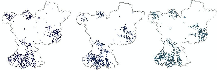
General plan
• Spatial questions
• Spatial data formats & types
• R packages for
  – Spatial data analysis
  – Map visualisation
• Research examples
  – Disease mapping
  – Web-based interpolation
  – Conservation planning
Spatial questions

• Metric space
  – How far? What direction? What area?...
  – Affected by map projection
  – Image processing, Vector graphics, CAD…
• Topological space
  – Connected? Within? Accessible from?
  – Graph theory, optimal routing…
Vector models of the world
• Coordinates: points, lines, polygons etc..
• Great for discrete, homogeneous objects.

© Crown Copyright/database right 2007 An Ordnance Survey/EDINA supplied service
Raster models of the world
• Regular sampling: ideal for continuous
  phenomena - aerial photo or a satellite image.
Vector and raster data in R

• Vector formats
  – Shapefiles, csv and text files…
• Raster formats
  – Geotiff, netCDF..

sp, rgdal, raster, maptools,
RArcInfo, ncdf
  fundamental data types and reading/writing
Spatial analysis in R
gstat, geoR, intamap, spacetime, akima
    spatial / spatiotemporal kriging / interpolation
rgeos
    topological operations: e.g.,intersection…
PBSmapping, maps, GEOmap, mapproj
    point-in-polygon, re-projection…
ecespa, spatstat, spatial, splancs
    point pattern analysis
trip, adehabitat, rangeMapper
    animal tracking and territory mapping
landsat
    topographic /other correction of satellite imagery
glmmBUGS, Mondrian, spdep, RPyGeo…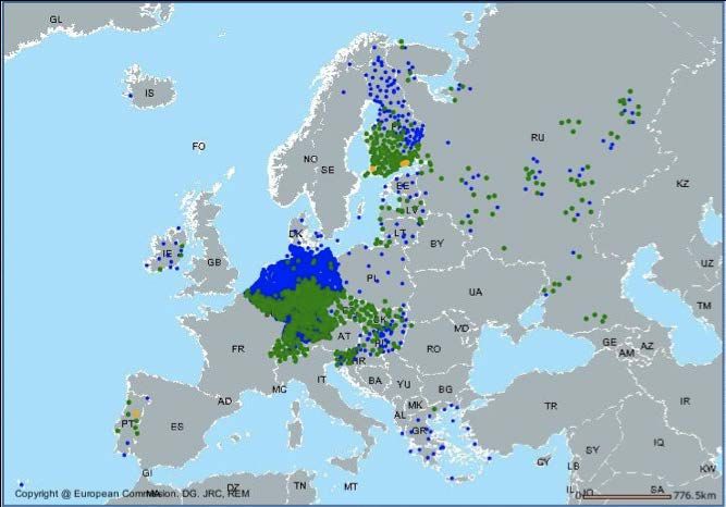
Visualisation in R
RgoogleMaps,plotKML,OpenStreetMap
    overlay data on Google Maps or OSM
ggmap (enhances ggplot2)
    overlay on Google Maps, Stamen, OSM or CloudMade
rasterVis
    interactive image mapping (esp. large rasters)
maps, GEOmap, rworldmap, GADM
    country boundary datasets & map functions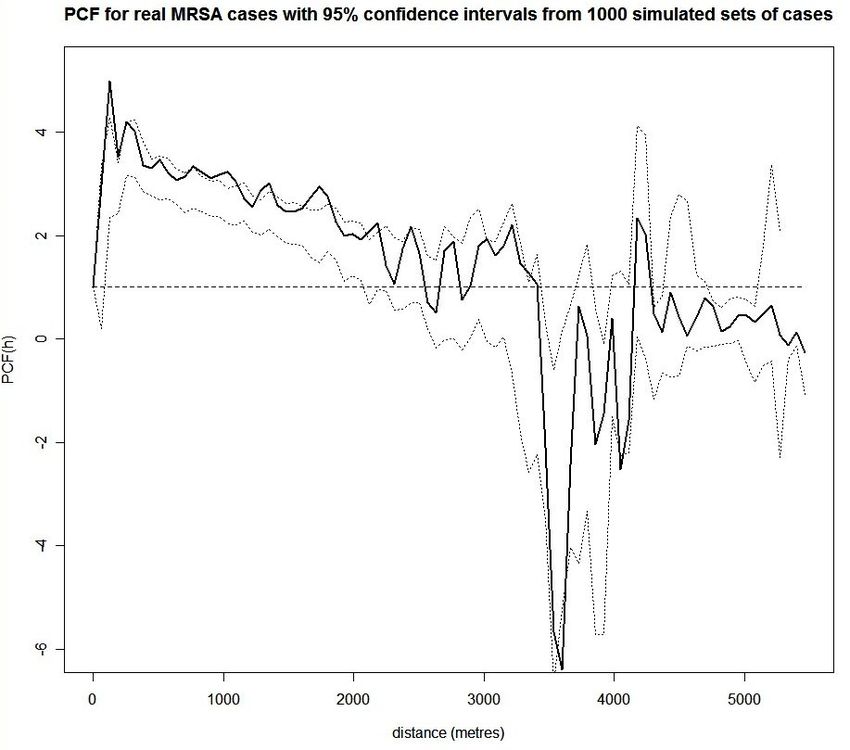
Claudia Engel: GADM example from
http://blog.revolutionanalytics.com/2009/10/geographic-maps-in-r.html
rworldmap

* http://journal.r-project.org/archive/2011-1/RJournal_2011-1_South.pdf
References, tutorials, etc.

http://www.bias-project.org.uk/ASDARcourse/unit7_slides.pdf
https://sites.google.com/site/rodriguezsanchezf/news/usingrasagis
http://www.itc.nl/~rossiter/teach/R/RSpatialIntro_ov.pdf

* https://dl.dropbox.com/u/24648660/ggmap%20useR%202012.pdf
http://www.nceas.ucsb.edu/scicomp/usecases/CreateMapsWithRGraphics
http://journal.r-project.org/archive/2011-1/RJournal_2011-1_South.pdf
http://geography.uoregon.edu/geogr/topics/maps.htm
http://www.milanor.net/blog/?p=594
http://spatialanalysis.co.uk/r/
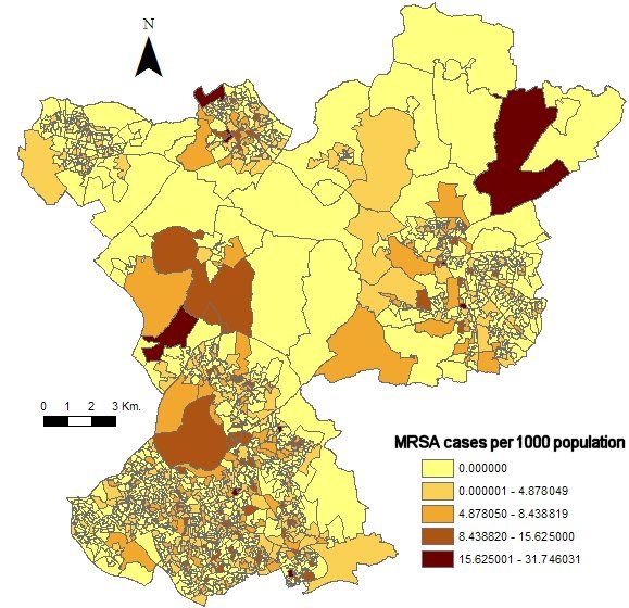
1. Disease mapping
• Working with local PCTs to map infection.
• Example: community-associated MRSA.
• Infections in people who have not recently
  visited a hospital as an in- or out-patient.
• Using demographic / environmental factors
  to identify SIGNIFICANT clusters of disease.
• R packages: splancs and spatstat
Simulating disease rates
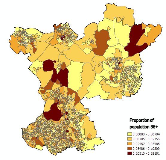
• Underlying population demographics
– E.g., differing susceptibility with age.
0.035
0.03
0.025
0.02
MRSA Ratio of MRSA to MSSA by age category
0.015 MSSA
1.2
0.01 1
0.8
0.005 0.6
0.4
0 0.2
0
29
44
59
64
74
84
us
o4
5
o1
pl
to
to
to
to
to
to
0t
5t
0to4 5to15 16to29 30to44 45to59 60to64 65to74 75to84 85plus
85
16
30
45
60
65
75Simulated disease cases Underlying population stratified by age and other risk factors Many realisations created (e.g., to model the expected patterns if infection was a random Poisson process free of spatial autocorrelation)
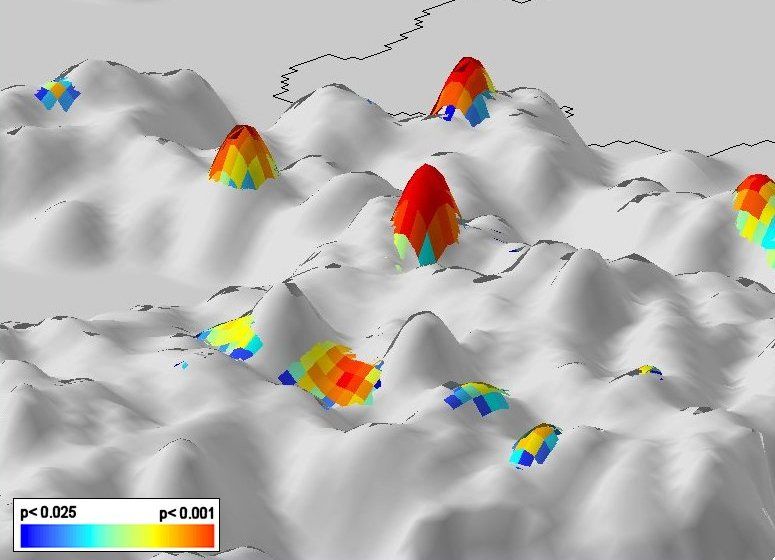
Disease mapping and modelling

   Using underlying data on sociodemographic and
   environmental factors to identify SIGNIFICANT
   clusters of disease – e.g., community-associated MRSA

These point realisations are
kernel-filtered, to produce density
grid maps that can be overlaid.
Disease          mapping
  Significant spatio-temporal clustersand modelling

Using underlying data on sociodemographic and
environmental factors to identify SIGNIFICANT
clusters of disease – e.g., community-associated MRSA

                                  Grey = 97.5th percentile
                                  of the simulated surfaces
Disease mapping and modelling
Using underlying data on sociodemographic and
environmental factors to identify SIGNIFICANT
Cluster locations investigated in detail:
clusters of disease – e.g., community-associated MRSA
- Unreported outbreaks at nursing homes.
- Infections in surrounding areas.
Bastin, Rollason, Hilton et. al (2007)
International Journal of GIS, 21 (7): 811-835.Specific genetic strains
of MRSA clustered in
specific areas of the
West Midlands.
Potential for tracking &
tracing infections which
move between hospital &
community
(e.g., C. difficile).
Ethical issues - patient
confidentiality!!!
Rollason, Bastin, Hilton et. al (2008)
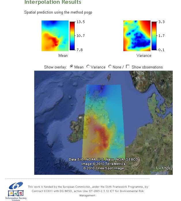
Journal of Hospital Infection, 70 (4): 314-202. Web-based interpolation • Real-time automatic mapping of environmental variables. • Web Services expose R algorithms to interpolate from point observations, with clearly-quantified reliability. • http://www.intamap.org • Used Java to interface with R, but…. • http://www.rstudio.com/shiny/
Case study – radiation
EURDEP radiation monitoring network

                                      Web Service for interpolating
                                      and mapping risk.
Sensor brand A:
Sensor networks - issues. Precision ± 0.3
No bias
Sensor brand B:
Gaussian error ± 0.8
Potential bias due
to elevation.
Sensor brand C:
Positive exponential
noise, varies with level.
Bias unknown.
Network is HETEROGENEOUS
in spatial pattern and accuracy
of measurements.
Projected sequential Gaussian process
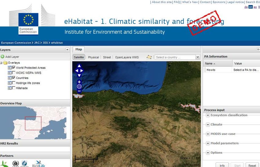
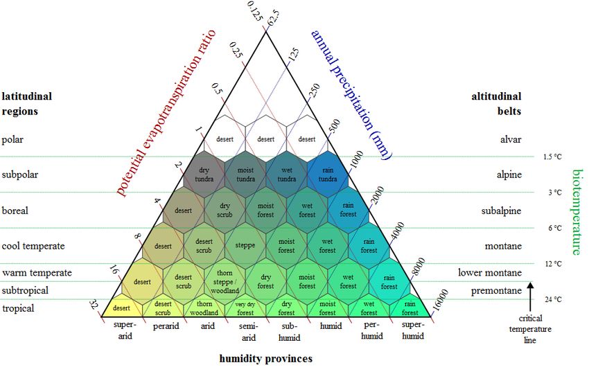
kriging (Cornford et al., StatGIS, 2009)3. Conservation planning • Select sites for protection based on their potential, now and in the future. • Data on species and available habitat is prone to error. • The future context may be hard to predict. • Can simulate various outcomes: climate change, development pressure, policy…
Identify species of interest

Example PA:
Ngorongoro
Species extent:
50% with most
restricted ranges
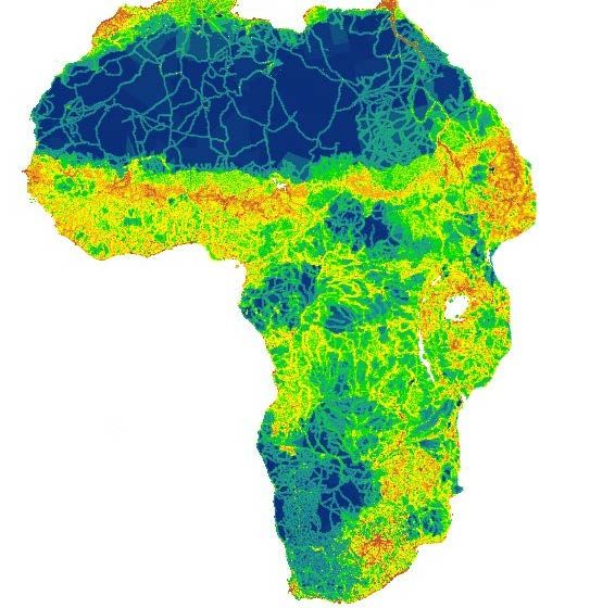
• Identify biome ‘envelope’
- Climatic variables from Holdridge’s lifezones
  (Biotemperature, precipitation, PET/precipitation)
Current

          2080
http://ehabitat-wps.jrc.ec.europa.eu/ehabitat/
You can also read