Spatial distribution, abundance, and management of fisheries in a changing climate
←
→
Page content transcription
If your browser does not render page correctly, please read the page content below
Vol. 668: 185–214, 2021              MARINE ECOLOGY PROGRESS SERIES
                                                                                                     Published June 24
https://doi.org/10.3354/meps13705                Mar Ecol Prog Ser

                                                                                                    OPEN
                                                                                                    ACCESS
REVIEW

          Antarctic krill Euphausia superba:
  spatial distribution, abundance, and management
           of fisheries in a changing climate
      Margaret M. McBride1,*, Olav Schram Stokke2, 3, Angelika H. H. Renner1,
Bjørn A. Krafft1, Odd A. Bergstad1, Martin Biuw1, Andrew D. Lowther4, Jan E. Stiansen1
                         1
                         Institute of Marine Research, PO Box 1870 Nordnes, 5817 Bergen, Norway
                          2
                            University of Oslo, Department of Political Science, 0317 Oslo, Norway
                                       3
                                        Fridtjof Nansen Institute, 1326 Lysaker, Norway
                         4
                           Norwegian Polar Institute, PO Box 6606 Langnes, 9296 Tromsø, Norway

      ABSTRACT: Antarctic krill Euphausia superba, a keystone species in the Southern Ocean, is
      highly relevant for studying effects of climate-related shifts on management systems. Krill pro-
      vides a key link between primary producers and higher trophic levels and supports the largest
      regional fishery. Any major perturbation in the krill population would have severe ecological and
      economic ramifications. We review the literature to determine how climate change, in concert
      with other environmental changes, alters krill habitat, affects spatial distribution/abundance, and
      impacts fisheries management. Findings recently reported on the effects of climate change on krill
      distribution and abundance are inconsistent, however, raising questions regarding methods used
      to detect changes in density and biomass. One recent study reported a sharp decline in krill den-
      sities near their northern limit, accompanied by a poleward contraction in distribution in the
      Southwest Atlantic sector. Another recent study found no evidence of long-term decline in krill
      density or biomass and reported no evidence of a poleward shift in distribution. Moreover, with
      predicted decreases in phytoplankton production, vertical foraging migrations to the seabed may
      become more frequent, also impacting krill production and harvesting. Potentially cumulative
      impacts of climate change further compound the management challenge faced by CCAMLR, the
      organization responsible for conservation of Antarctic marine living resources: to detect changes
      in the abundance, distribution, and reproductive performance of krill and krill-dependent preda-
      tor stocks and to respond to such change by adjusting its conservation measures. Based on
      CCAMLR reports and documents, we review the institutional framework, outline how climate
      change has been addressed within this organization, and examine the prospects for further
      advances toward ecosystem risk assessment and an adaptive management system.

      KEY WORDS: Antarctic krill · Climate change · Ecosystem · Distribution · Abundance · Food web ·
      Management · CCAMLR · Commission for the Conservation of Antarctic Marine Living Resources

                 1. INTRODUCTION                               ronmental conditions, respond quickly to ecosystem
                                                               perturbations (Flores et al. 2012a, Rintoul et al. 2012,
  The Southern Ocean is a region of high physical              De Broyer et al. 2014, McBride et al. 2014). Climate
and biological variability (Hempel 1985, Constable et          change may affect organisms and populations physi-
al. 2003). Its diverse biota, adapted to extreme envi-         ologically and by altering their habitats. Understand-
                                                               © The authors and Research Council of Norway 2021. Open Access
*Corresponding author: margaret.mcbride@hi.no                  under Creative Commons by Attribution Licence. Use, distribution
                                                               and reproduction are unrestricted. Authors and original publication
                                                               must be credited.
                                                               Publisher: Inter-Research · www.int-res.com
186                                          Mar Ecol Prog Ser 668: 185–214, 2021

ing these habitat effects facilitates understanding the           CCAMLR’s approach to krill fisheries management
effects on biological variables such as population dis-           to accommodate ongoing and future climate-related
tribution, abundance and movement patterns, and                   changes in the stock? We synthesize the results of
biomass production. Possible shifts in the distribution           studies published in peer-reviewed journals to pro-
of commercially harvested Antarctic krill Euphausia               vide an overview of changes in the physical and bio-
superba (henceforth krill) populations in response to             logical environment and examine how these changes
climate variability present a key challenge to effec-             affect the distribution and abundance of krill. Based
tive management.                                                  on CCAMLR reports and documents, we examine
   The Commission for the Conservation of Antarctic               how climate change has been addressed within this
Marine Living Resources (CCAMLR) has established                  organization, with an emphasis on its ecosystem-based
precautionary catch limits on the krill fishery in most           risk assessment of krill fisheries and its advances
of the areas where fishing has occurred, but these                toward a feedback management system capable of
catch limits apply to large statistical subareas. It is           responding to climate variability.
now 3 decades since the CCAMLR stated its ambi-
tion to advance from a precautionary approach to a
feedback management system capable of continu-                           2. KRILL BIOLOGY AND PHYSICAL
ously adjusting krill conservation measures in re-                                ENVIRONMENT
sponse to new knowledge on krill stocks and associ-
ated species (CCAMLR 1991a). However, monitoring                                       2.1. Biology
of krill stocks and krill-dependent species has been
too limited to provide a satisfactory knowledge base                Antarctic krill (Fig. 1, Table 1) is a large (up to
to assess the level of risk associated with krill fish-           65 mm), long-lived (5−7 yr lifecycle) euphausiid spe-
eries and respond quickly to changing indices of eco-             cies that is abundant, widely distributed, and ecologi-
system components — including updated, lifecycle-                 cally important in the Southern Ocean. It can form
sensitive, and spatially relevant information on krill            large swarms, sometimes reaching densities of 10 000−
distribution, abundance, flux, and trophic inter-                 30 000 ind. m−3 (Hamner et al. 1983). Its biology and
actions (Krafft et al. 2015, 2018, BAS 2018, Santa                ecology have been reviewed many times: in multi-
Cruz et al. 2018). CCAMLR has recognized the need                 authored publications (e.g. Everson 2000, Siegel 2016);
for revision of current management approaches as                  in numerous scientific publications (e.g. Bargmann
urgent (CM 51-07-2016; CCAMLR 2016b).                             1945, Marr 1962, Cuzin-Roudy & Amsler 1991, Atkin-
   This review seeks to answer 2 main questions: (1)              son et al. 2004, 2008, 2019, Kawaguchi & Nicol 2007,
What are the potential cumulative effects of climate              2020, Siegel & Watkins 2016, Cox et al. 2018); and as a
change on the distribution and abundance of Antarc-               popular science book (Nicol 2018). Rather than repeat
tic krill? (2) What are the prospects for changing                what has already been reported, this section focuses
                                                                  on aspects of krill biology which make it vulnerable to
                                                                  climate-related changes in its physical environment.
                                                                    Antarctic krill is a cold-adapted stenothermic spe-
                                                                  cies mainly inhabiting waters < 3.5°C; sudden water
                                                                  temperature changes might impact its physiological
                                                                  performance and behavior (Daly 1998, Flores et al.
                                                                  2012a, Krafft & Krag 2015). During the course of its
                                                                  complicated life cycle, krill inhabits benthic, surface,
                                                                  and pelagic environments structured by sea-ice
                                                                  extent and concentration, water temperatures, and
                                                                  circulation patterns (Nicol 2006, Nicol & Raymond
                                                                  2012). Its annual and lifecycle phases occur in close
                                                                  association with sea ice, where it feeds on ice algae
                                                                  and finds shelter from predators (Quetin & Ross 2001,
                                                                  Brierley et al. 2002, Smetacek & Nicol 2005) (Fig. 2).
Fig. 1. Pelagic female Antarctic krill feeding on summer phyto-     Piñones & Fedorov (2016) identified 3 critical peri-
plankton. Adults range from 5.0 to 6.5 cm in length and weigh
                                                                  ods of the krill early lifecycle during which environ-
an average of 2 g. Adult females are slightly larger than adult
males. Image © V. Siegel, Thünen Institut für Seefischerei,       mental conditions exert a dominant control over sur-
                Hamburg, used with permission                     vival: (1) development of larvae into the first feeding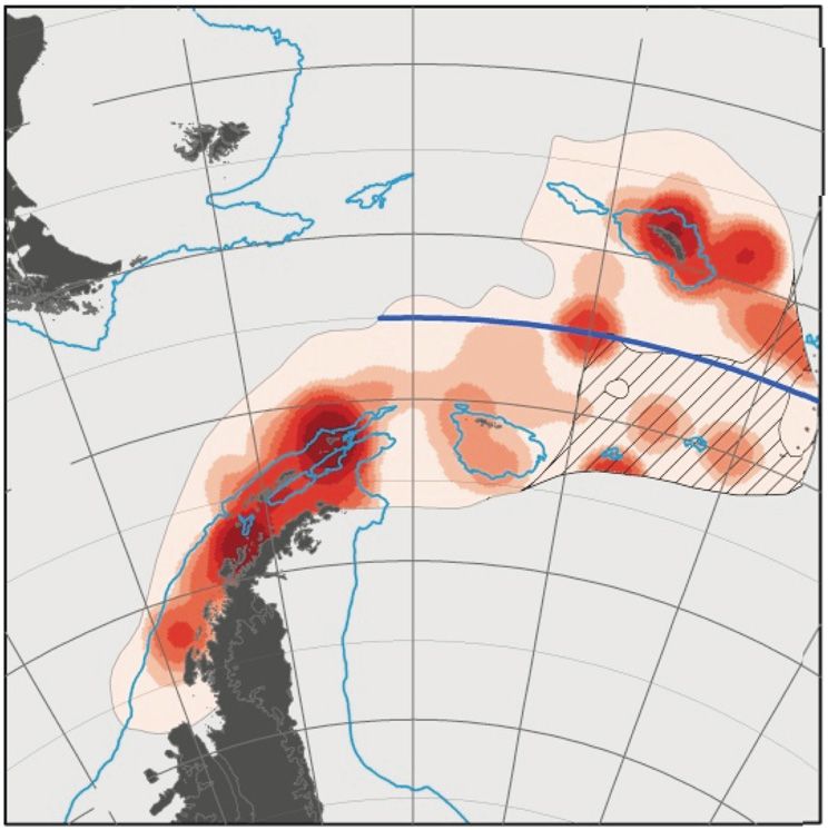
McBride et al.: Antarctic krill, climate change, and fisheries management                            187

Table 1. Biological characteristics of Antarctic krill living in the Southern Ocean south of the Antarctic Polar Front (adapted
                                                   from: De Broyer et al. 2014)

 Biological characteristic                    Reported observation                                  References

 Vertical depth range (m)                    Surface to 3000                                   Taki et al. (2008)
 Temperature range (°C)                          −1.8 to 5                         Ross et al. (2000), Schmidt et al. (2014)
 Swarming behavior                                   +                                      Ross & Quetin (2000)
 Vertical migration                                  +                                         Taki et al. (2008)
 Adult size (mm)                                     65                                     Ross & Quetin (2000)
 Adult weight (g)                                     2                                     Ross & Quetin (2000)
 Lifespan (yr)                                     5−7                              Siegel (1987), Ross & Quetin (2000)
 Spawning period (cycles)                December−April (1 to 3)                   Mauchline (1980), Ross & Quetin (2000)
 Diet (adults)                     Phytoplankton (diatoms, flagellates),        Mauchline & Fisher (1969), Phleger et al. (2002)
                                     zooplankton (copepods), detritus
 Predators                            Whales, seals, birds, fish, squid              Nemoto et al. (1985), Murphy et al. (2016)

stage at the end of austral summer; (2) accumulation                   2016). Projected reduction in sea-ice coverage (~80%
of sufficient lipid reserves during late summer and                    by 2100) may reduce krill spawning grounds in
fall, allowed by food availability; and (3) enduring the               important habitats such as along the west Antarctic
first winter, when under-sea ice habitat provides both                 Peninsula in the southwest Atlantic sector (Hofmann
food (algae) and shelter (Fig. 2). Temperature and                     et al. 1992, Fach et al. 2002, 2006, Thorpe et al. 2004,
depth of Circumpolar Deep Water control success of                     2007, Atkinson et al. 2008, Piñones et al. 2013, Piñones
the descent−ascent phase of the krill reproductive                     & Fedorov 2016).
cycle (Quetin & Ross 1984, Hofmann & Hüsrevoğlu
2003); temperature also moderates the extent of sea
ice (Daly 1990, Ross & Quetin 1991, Meyer et al. 2002).                               2.2. Physical environment
   The winter under-ice population is dominated by
larvae and juvenile krill feeding on the available ice                   Circulation in the Southern Ocean is dominated by
algae. Consequently, sea-ice retreat, particularly in                  the eastward-flowing Antarctic Circumpolar Current
winter, can become a dominant driver of krill popula-                  (ACC). Closer to the coast, the Antarctic Coastal Cur-
tion decline (Flores et al. 2012a,b, Piñones & Fedorov                 rent flows westward around the continent. The other

                             Summer                         Fall                      Winter                         Spring
–1 0 1 2°C
                                                                               SIB             Sea Ice                          0m

           Female                        C1

                                                                                                         Juveniles
                                              Chl a           Larvae                                                          200 m

 CDW
                    Embryo
                                                                                                                                      Depth

                                   CP1                CP2                       CP3

                                                                                                                              800 m
                          Hatching

                       Sea floor
Fig. 2. Antarctic krill early lifecycle. After hatching, embryos develop from nauplii to first feeding stage calyptopis 1 (CP1); af-
ter the descent/ascent cycle (CP1), they feed on chlorophyll a (chl a) during summer and early fall. They overwinter under-
neath sea ice and molt into juveniles in spring. Three critical periods (CP1, -2, and -3) are indicated. SIB: sea-ice biota for win-
ter-feeding by krill larvae. CDW: Circumpolar Deep Water. (Source: modified figure and description used with permission
                                                    from Piñones & Fedorov 2016)
188                                        Mar Ecol Prog Ser 668: 185–214, 2021

                                                               Temperature increase in the Antarctic Bottom Water,
                                                               together with a freshening (Azaneu et al. 2013, Jul-
                                                               lion et al. 2013), has resulted in a contraction of its
                                                               volume (Purkey & Johnson 2012, Azaneu et al. 2013).
                                                               On the shelf, Schmidtko et al. (2014) found a complex
                                                               pattern of temperature trends in Antarctic Continen-
                                                               tal Shelf Bottom Water, with regional patterns of
                                                               warming along most of the Antarctic Peninsula and
                                                               in the Bellingshausen and Amundsen Seas, and cool-
                                                               ing in the southern Weddell Sea.
                                                                  SST and specific isotherms are often used to iden-
                                                               tify positions of the ACC front. Following such defini-
                                                               tions, observed warming implies a potential pole-
                                                               ward shift of the ACC and its fronts (Gille 2008,
                                                               Cristofari et al. 2018). However, fronts are more com-
                                                               plex than their SST expression, and more advanced
Fig. 3. Projected summer (January to March) sea surface
                                                               analyses have not revealed such a shift (Gille 2014,
temperature (SST) anomaly for the region between 0° and
90°W and south of the Antarctic Polar Front (Antarctic Con-    Freeman et al. 2016, Chapman 2017, Chambers
vergence). The SST anomaly is the annual mean of spatially     2018). Future projections of ACC strength, meander-
resolved summer SSTs for a specific model realization minus    ing, and position involve considerable uncertainty
the 1991−2020 mean of spatially resolved summer SSTs for       (Meijers et al. 2012, 2019, Meijers 2014). Any such
the same model realization. The colored lines indicate the
mean SST anomaly for 1991−2099 across all available models     changes in the ACC, as well as changes in ocean
for each of 3 Representative Concentration Pathways (RCPs),    temperatures, might influence the volume and stabil-
and the shaded envelopes indicate the between-realization      ity of Antarctic sea ice (Gille 2002).
standard deviation for RCPs 2.6 and 8.5. (Source: figure and      By reducing the area of sea-ice formation near the
    description used with permission from Hill et al. 2013)
                                                               Antarctic Peninsula and other critical regions of the
                                                               Southern Ocean, climate change is reducing the
major physical feature of this system is the annual            feeding potential for krill and, consequently, its
advance and retreat of sea ice (Constable et al. 2003).        recruitment and overall production (Walther et al.
Parts of the Southern Ocean warmed considerably                2002, Flores et al. 2012a,b). The central role of krill in
during the second half of the 20th century, with               Southern Ocean food webs makes understanding
greater temperature increases in some regions than             how climate affects its abundance and distribution a
those of the global ocean (Fig. 3) (Levitus et al. 2000,       prerequisite for effective management of commercial
2005, Gille 2002, 2008, Whitehouse et al. 2008,                fisheries. Particularly, the rapid rate of changes
Schmidtko et al. 2014, Swart et al. 2018).                     underway in the Antarctic marine ecosystem neces-
  Particularly the Atlantic sector of the Southern             sitates better predictions of how inter-annual vari-
Ocean, where most krill is located, has experienced            ability in environmental conditions may influence
rapid upper-ocean warming (Meredith & King 2005,               krill production and affect krill-dependent species.
Whitehouse et al. 2008), loss of winter sea ice (Parkin-
son 2002), and great inter-annual variability in chloro-
phyll a (chl a) concentrations (Constable et al. 2003).          3. CLIMATE-CHANGE IMPACTS ON SPATIAL
Summer foraging sites for krill in the Atlantic sector           DISTRIBUTION AND ABUNDANCE OF KRILL
have experienced sea surface temperature (SST) in-
crease of up to 0.2°C per decade, and projections indi-          After nearly a century of observations, the general
cate that further widespread increase of 0.27−1.08°C           patterns of krill occurrence and distribution have
per decade may occur by the late 21st century (Fig. 3)         been determined. Krill distribution exhibits consider-
(Hill et al. 2013). This warming trend is not spa-             able spatial variability, both inter- and intra-annual,
tially uniform, however; certain parts of the Southern         with juveniles and adults forming large swarms
Ocean are cooling (Gille 2008, Schmidtko et al. 2014).         (Nicol et al. 2012, Siegel & Watkins 2016, Ryabov et
  Off the continental shelf, Circumpolar Deep Water            al. 2017, Atkinson et al. 2019). They perform large
has warmed in most regions (Gille 2008, Schmidtko              horizontal and vertical migrations (from surface to
et al. 2014), with similar warming below 2000 m                > 3000 m depth) (Morris et al . 1983, Kawaguchi &
(Purkey & Johnson 2012, Desbruyères et al. 2016).              Nicol 2007, De Broyer et al. 2014). H owever, less is
McBride et al.: Antarctic krill, climate change, and fisheries management                            189

known of the precise migration patterns, as much of            krill genetic and genomic data had not indicated
the Southern Ocean is still poorly sampled. There              genetic structuring of krill by sites around Antarc-
is concern over possible long-term changes in krill            tica. In contrast, Clarke et al. (2021) indicated that
distribution and abundance as a result of climate              krill-associated bacterial communities are geograph-
change and harvesting, and how to distinguish these            ically structured.
variables from each other in time and space (Siegel &             The horizontal distribution of krill is affected by
Watkins 2016).                                                 advection and retention due to ocean currents,
  Richardson (2008) suggested that mechanisms re-              eddies, and sea-ice drift, depending on hydrody-
lated to climate change and the retreat of sea ice will        namic forces and stage in the krill lifecycle (Nicol
primarily impact krill in 3 ways:                              2006, Mori et al. 2017). Larval and juvenile krill are
  (1) Water temperature in correlation with sea ice            passively advected by prevailing currents. Although
coverage appears to be the driving factor for krill            adult krill are strong swimmers, capable of going
density (Trathan et al. 2003, Wiedenmann et al. 2008,          against the currents, their movements are influenced
2009, Wiedenmann 2010). In warming regions of the              by the flow regime around individuals and swarms
Southern Ocean, a negative relationship between                (Tarling & Thorpe 2014, Reiss et al. 2017). Within a
increasing surface temperature and krill density has           flow regime where surface current speeds can reach
already been observed (Trathan et al. 2003, Atkinson           up to ca. 100 cm s−1 (Smith et al. 2010, Tarling &
et al. 2019).                                                  Thorpe 2014), individual adult krill can maintain
  (2) There may be changes in the timing of important          speeds of no more than 15 cm s−1 without increasing
events in the krill lifecycle (phenology), such as the         metabolic rate (Kils 1981); this may limit their capac-
timing of spawning or hatching (Wiedenmann 2010).              ity to control their location within highly advective
  (3) Levels of abundance may change, mediated                 environments. Krill swarms sustain speeds of 20 cm
largely through variable food supply. However, de-             s−1 (Hamner 1984, Tarling & Thorpe 2014); this may
tecting long-term trends in abundance and attribut-            help to maintain swarm coherence in the face of dis-
ing them to climate variation is more difficult than           persive surface currents (Zhou & Dorland 2004).
detecting the changes described above (Wieden-
mann 2010).
  Other potentially important mechanisms include:
  (4) The effect higher temperatures have on individ-
ual growth. Krill grow through a series of molts, and
both the time between molts and growth increment
per molt are inversely temperature-dependent
(Quetin et al. 2003, Atkinson et al. 2006, Kawaguchi
et al. 2006, Tarling et al. 2006, Wiedenmann 2010,
Bellard et al. 2012).
  (5) The direct impact of the changing seasonal
cycle of light on krill physiological processes, such as
initiation of production of oocytes (Spiridonov 1995,
Quetin et al. 2007).

      3.1. Impacts on horizontal distribution

  Mackintosh (1973) indicated 5 to 6 krill stocks
around the Antarctic continent but suggested that
these areas of higher krill density should not be
regarded as isolated populations. Latogurski (1979)
speculated that krill associated with the 3 main gyre
systems around the continent might be regarded as
independent populations (Duan et al. 2016, Siegel &            Fig. 4. Observed distribution and concentration of Antarctic
                                                               krill (ind. m−2 within each 5° longitude by 2° latitude grid cell,
Watkins 2016), but the vast population size and huge           ND: no data, 0*: no Antarctic krill recorded in the available
genome make it difficult to detect separate krill              data). (Source: modified figure and description used with
stocks. Deagle et al. (2015) reported that studies of          permission from Atkinson et al. 2008 and Hill et al. 2013)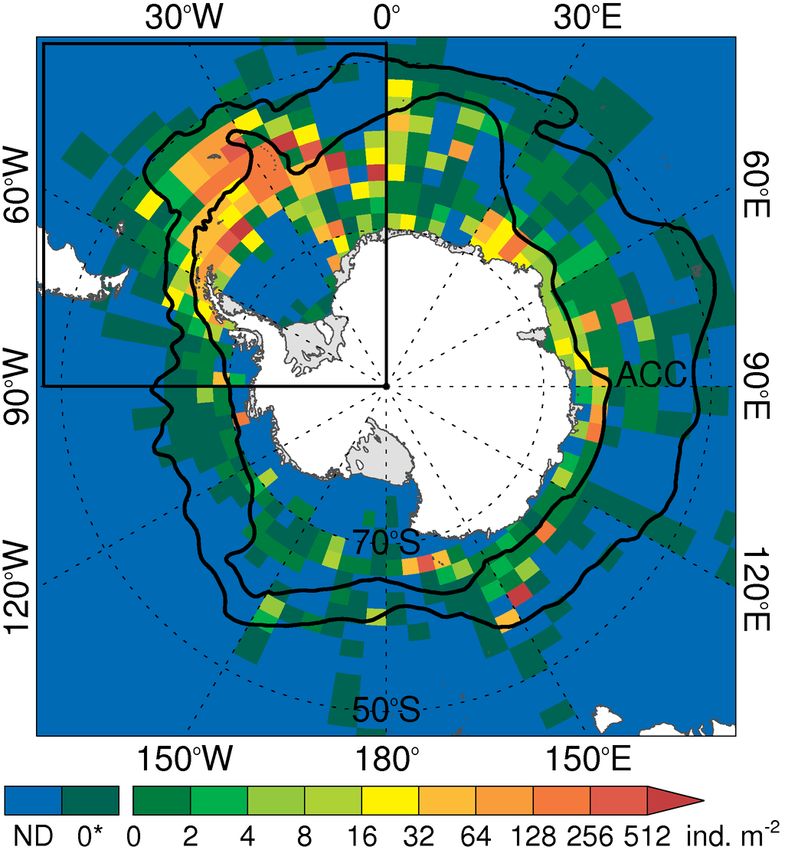
190                                      Mar Ecol Prog Ser 668: 185–214, 2021

      3.1.1. Ocean warming and habitat quality               (Atkinson et al. 2004). At the physiological level, high
                                                             phytoplankton concentration can sometimes com-
   The habitat used by krill comprises more than half        pensate for the negative effects of temperature (Pört-
of the approximately 32 million km2 area of the entire       ner 2012). This is demonstrated by elevated krill
Southern Ocean south of the Polar Front (Mackintosh          abundance and favorable growth rates observed at
1973, Siegel & Watkins 2016). The horizontal distri-         South Georgia. This area is near the northern limit of
bution of krill is uneven, however, with more than           the species’ range; it has relatively high and physio-
half of the circumpolar population occurring in the          logically stressful temperatures, but also has very
Atlantic sector (Atkinson et al. 2004) (Fig. 4). The         high food concentrations (Atkinson et al. 2008). Qual-
largest concentrations and highest densities (ob-            itative analyses of krill habitats have consistently
served and predicted) occur around the Antarctic             shown that spatio-temporal variability is a common
Peninsula, in the Scotia and Weddell Seas — particu-         feature of krill populations and that krill habitat can-
larly in the Polar Front zone and the Southern ACC           not be simply described using a small number of vari-
Front — and from the continental coast to the north-         ables (Jarvis et al. 2010, O’Brien et al. 2011, Young et
ern limit of the Polar Front in the whole eastern sec-       al. 2014).
tor (Marr 1962, Atkinson et al. 2004, Nicol 2006, De            Diatom blooms provide an essential food for the
Broyer et al. 2014, Siegel & Watkins 2016, Silk et al.       lipid metabolism of krill (Mayzaud et al. 1998): energy
2016). Data from comparable net and acoustic sur-            transfer from these spring phytoplankton blooms is
veys indicate that average krill densities in the South      essential for sexual differentiation in gonads during
Atlantic may be 10 times higher than off East Antarc-        the late furcilia phase of larval development (Cuzin-
tica (30−150°E) (Nicol et al. 2000a,b, Nicol 2006); this     Roudy 1987a,b); maturation into adulthood, the onset
region, with its convoluted coastline and many island        of successive reproductive cycles during summer
groups, offers more suitable habitat for krill (Nicol        (Cuzin-Roudy 1993, 2000); and maintaining high
2006, Atkinson et al. 2008). Despite high concentra-         fecundity during summer (Cuzin-Roudy & Labat
tions in the Atlantic sector, the habitat used by krill      1992, Ross & Quetin 2000).
comprises more than half of the approximately 32                Employing models that explicitly include the inter-
million km2 area of the entire Southern Ocean south          acting ecological effects of temperature and food
of the Polar Front (Mackintosh 1973, Siegel &                availability is a useful step towards fuller considera-
Watkins 2016).                                               tion of the multiple interacting effects of climate
   The circumpolar distribution of krill has been ob-        change on the abundance and distribution of krill
served from the continent to the northern limit of the       (Stock et al. 2011, Pörtner 2012, Hill et al. 2013).
Polar Front, although in most of their range they are
far to the south. The only region where krill was —
both observed and predicted to be — absent in the                               3.1.2. Poleward shift
entire Polar Front Zone lies between 60 and 150°E
(De Broyer et al. 2014). In this region, sea ice retreats      Modeling studies to predict the fate of krill under
almost completely to the coast during summer, and            different warming scenarios seem to be in general
hydrographic conditions are different. Low concen-           agreement, forecasting both a reduction and a pole-
trations of silicates (which do not favor diatom             ward shift of the available krill habitat for spawning
blooms) and climate-induced changes in the mixed-            and growth (Hofmann et al. 1992, Hill et al. 2013,
layer depth (which affect both spatial distribution of       Cuzin-Roudy et al. 2014, CCAMLR 2015, Piñones &
production and phytoplankton commu nity structure)           Fedorov 2016). The Cuzin-Roudy et al. (2014) model
are likely driving factors behind the reduced occur-         of habitat suitability explained 63% of variance and
rence of krill in this region, as the best habitat condi-    has been used to infer the presence of krill in regions
tions generally occur near the continental shelf (Flo-       where sampling data are limited (Fig. 5). The results
res et al. 2012a).                                           show high probability of occurrence almost every-
   Suitable krill habitat is linked to various pro-          where south of the Polar Front, and low probability
cesses — seasonal sea-ice dynamics, frontal zones,           north of it (Cuzin-Roudy et al. 2014). Habitat model-
and mixing associated with bathymetry (Siegel 2005,          ing also indicates that, at high latitudes, horizontal
Murphy et al. 2007), spring light regime, and supply         distribution and spawning may extend to areas of
of critical nutrients like nitrates and iron — support-      suitable habitat where krill has not been observed in
ing the production of chl a, an important indicator of       the past, including in the Indian Ocean and Pacific
the presence and concentration of phytoplankton              sectors (Atkinson et al. 2008).
McBride et al.: Antarctic krill, climate change, and fisheries management                      191

                                                             0°

                              30°W                                                      30°E
                                                           45°S

                                                           55°S

          60°W                                                                                              60°E
                                                           65°S

                                                           75°S

  90°W                                                                                                              90°E

          120°W                                                                                            120°E

 Legend
 Value
         High : 1             150°W                                                    150°E

         Low : 0                                           180°

Fig. 5. Antarctic krill modeled habitat suitability using presence/absence data and environmental variables. (Source: figure
                              and description used with permission from Cuzin-Roudy et al. 2014)

   However, less attention has been paid to actual                and water-mass distribution. High SAM values ap-
measurement of latitudinal shifts in the range of krill           pear to be associated with low krill densities during
distribution. Using mixed models and a data time-                 the modern era (1976 to present) and across the
series derived from the KRILLBASE project (Atkin-                 southwest Atlantic sector (Atkinson et al. 2019). It is
son et al. 2017), Atkinson et al. (2019) found that               likely that the SAM influences annual recruitment of
within the main population center, Antarctic krill dis-           small (< 30 mm) krill to the population through its
tribution has shifted southward (~440 km) over the                influence on factors that determine high or low
past 90 yr (Fig. 6a). They linked this response to vari-          phytoplankton production: air and sea temperature
ation in the Southern Annular Mode (SAM); this                    (Clarke et al. 2007), duration and extent of sea-ice
index is strongly correlated with both sea-ice extent             cover (Siegel & Loeb 1995), cloud cover, wind condi-
192 Mar Ecol Prog Ser 668: 185–214, 2021
a b North of 60° S
Low data area 40°W 5
Data not plotted 50°S All stations
South Georgia
Annual mean
Mean latitude: 4
57.3°S
52.5
3
log10 (krill density, number m –2)
55.0
Latitude (°S)
57.5 2
la
6 0°S su
in
60.0
en
1
cP
62.5
rc ti
A nt a
65.0 0
70°S
0 250 500
1926–1939 67.5
km 0 100 200 –1
Krill density (number m –2)
60°W 40°W
–2
50°S
Mean latitude:
57.5°S –3
52.5
1970 1980 1990 2000 2010 2020
55.0
Year
57.5
Latitude (°S)
60°
S South of 60° S
60.0 5
All stations
62.5 Annual mean
4
65.0
1976–1995 3
log10 (krill density, number m –2)
S 67.5
70° 0 100 200 300
Krill density (number m –2)
60°W 40°W 2
50°S
Mean latitude: 1
61.2°S
52.5
0
55.0
57.5
Latitude ( S)
–1
S
60° 60.0
–2
62.5
65.0 –3
1970 1980 1990 2000 2010 2020
1996–2016 Year
S 67.5
70° 0 10 20 30 40 50
Krill density (number m –2)
Fig. 6. Southward contraction of krill distribution within the SW Atlantic sector. (a) Kernel analysis visualizing hotspots of krill
density in the SW Atlantic sector during the Discovery sampling era (1926−1939) and the first and second halves of the modern
era, based on the area sampled heavily across all 3 periods. Blue isobaths denote the 1000 m boundary between shelf and
oceanic habitats. Within each map, the kernel analysis identifies relative hotspot areas of high density, signified by the inten-
sity of red shading. For a quantitative analysis, the histograms denote the mean density of krill in 6 comparable 2.5° latitude
bands with > 50 stations sampled in each era. Note changes in scale. Thick blue lines across maps and histograms indicate the
center of krill density (i.e. density-weighted mean latitude). (b) Trends in log10-transformed mean standardized krill density
north and south of 60° S. Small points represent the densities in underlying records; large dots represent the annual means of
these data, weighted by the number of stations per record. Pink dots represent seasons with < 50 stations (average 27 com-
pared to an overall average of 123 stations per season). Solid blue trend lines were fitted using simple linear regression (p <
0.001, p < 0.01 adjusted R2 = 0.52, 0.22 for north and south of 60° S, respectively). (Source: figure and description used with
permission from Atkinson et al. 2019)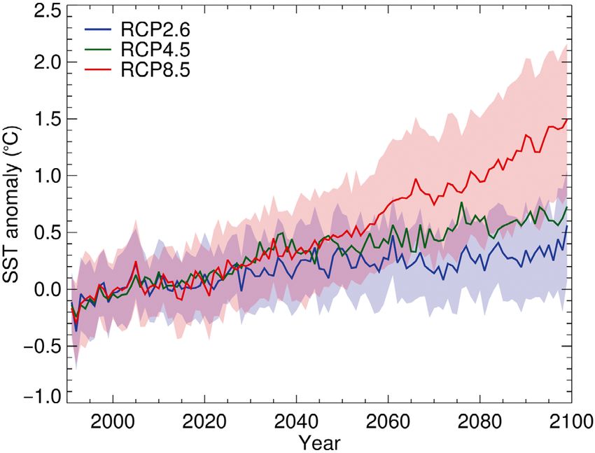
McBride et al.: Antarctic krill, climate change, and fisheries management                    193

tions (Wiedenmann et al. 2008), currents/circulation           plex than a simple poleward shift in distribution in
patterns, stratification, and advection (Flores et al.         response to increasing temperatures. Coastal embay-
2012a, Renner et al. 2012, Youngs et al. 2015).                ments and high-latitude shelves may serve as re-
   The ongoing trend towards positive SAM — most               fuges for growth but are unlikely to provide appro-
notably around the Antarctic Peninsula and periph-             priate habitats for spawning (Hofmann & Hüsrevoğlu
eral seas (Kwok & Comiso 2002) — means warmer,                 2003), or connectivity for subpopulations (Siegel 2005).
windier, and cloudier weather, and loss of sea ice
within the Southwest Atlantic sector, all of which neg-
atively affect krill feeding conditions. This adversely                    3.1.3. Diminished krill habitat
affects early spawning in spring, early larvae in sum-
mer, and later larval stages which need early form-               If a poleward shift in krill distribution has occurred,
ing, complex, and well-illuminated marginal sea ice            as argued by Atkinson et al. (2019), this is likely the
to promote survival (Meyer et al. 2017). Atkinson et           coping response of a physiologically stressed organ-
al. (2019) reported that krill densities near the north-       ism to a rapidly changing environment. Such adjust-
ern range limit have declined sharply: the population          ments in species habitat may not meet the require-
has become more concentrated in the south, where               ments for a population to persist, due to complex
continental shelf habitat is more extensive. They              interactions among animal behavior, advection, and
noted that krill density shows a strongly negative             retention to maintain populations in specific regions
trend north of 60° S and a weaker trend further south          (Hofmann & Murphy 2004). Various aspects of the
(Fig. 6b) and argued that SAM appears to be the                changed environment (e.g. temperature, availability
clearest predictor at the whole Southwest Atlantic             and quality of food) will affect individual growth,
scale. The El Niño−Southern Oscillation (ENSO) is              reproductive success, survival rate, and recruitment
also identified as a driver of krill dynamics near the         success, as well as our ability to fully determine habi-
Antarctic Peninsula (Loeb et al. 2009). The interplay          tat requirements (Walther et al. 2002, Quetin et al.
between SAM and ENSO strongly affects advection                2007).
patterns and outflow from the northwestern Weddell                One obvious aspect of a poleward shift in krill dis-
Sea — influencing the advection of nutrients, phyto-           tribution is the inferred contraction into diminished
plankton, and krill towards either the western                 habitat space — due to the meridians converging
Antarctic Peninsula or towards South Georgia via the           most rapidly at high latitudes — while further retreat
South Orkney Islands (Loeb et al. 2009, Renner et al.          is blocked by the continent itself (Atkinson et al.
2012, Youngs et al. 2015).                                     2019). Such a shift may also involve declines in bio-
   The findings of Atkinson et al. (2019) (Fig. 6) agree       mass and quality of phytoplankton food resources
with predictions of poleward shifts in species distri-         (Montes-Hugo et al. 2009), with negative impacts on
bution made by the Intergovernmental Panel on Cli-             feeding conditions, spawning success, and survival
mate Change (IPCC 2007). Uncertainties remain,                 of larvae. The exact mechanisms are likely to vary
however. For example, recent studies by Cox et al.             with latitude (Meyer et al. 2017).
(2018, 2019) — based on the same KRILLBASE data-                  Quetin et al. (2007) noted 2 additional potentially
set used by Atkinson et al. (2019) and Hill et al.             important aspects of sustainable habitat relative to a
(2019) — found no evidence of long-term decline in             poleward shift in krill distribution. Firstly, changes in
krill density or biomass, nor did they report a pole-          latitude determine the seasonal cycle of light, and
ward contraction of distribution in the Southwest              variation in the timing and amount of energy input
Atlantic sector. Contrasting results from these 2 stud-        into the ecosystem. The timing of ice formation at a
ies regarding long-term changes in krill density and           specific latitude is crucial to the amount of food avail-
biomass may be due to fundamental differences in               able to larval krill in their winter ice habitat. How-
how these researchers pre-processed and trans-                 ever, due to the differences in day length and sun
formed the data prior to submitting them to their              angle, the amount of solar energy reaching the Earth’s
respective modeling approaches, how log transfor-              surfaces in autumn and winter is significantly less at
mations were carried out, and statistical treatment of         higher latitudes. For organisms that can survive the
datasets. A fuller assessment of temperature effects           autumn and winter with some light, but not total
might consider how the relationship between SST                darkness, this decrease in light input may be critical.
and the temperatures experienced by krill through-             Secondly, the changing seasonal light cycle might
out the water column changes over time and space.              directly impact krill physiology. This area of research
The environmental effects are likely to be more com-           on krill ecology has not received much attention.

194                                      Mar Ecol Prog Ser 668: 185–214, 2021

However, over the latitudinal range where krill are          titioning within the population and contributes to the
found, there may be differences related to seasonal          flexibility and overall success of the species (Schmidt
shifts in the day/night light cycle: in behaviors such       et al. 2011).
as the periodicity of diel vertical migration (Gaten et         Early acoustic measurements were largely restricted
al. 2008); or in the timing of physiological processes       to depths ranging from 10 to 200 m, and net collec-
such as the initiation of oocyte production (Spiri-          tions were derived from tows over the upper 120 m.
donov 1995).                                                 Consequently, krill abundance in deeper waters can-
                                                             not be estimated using these datasets. Lascara et al.
                                                             (1999) suggested that the downward migration of
        3.2. Impacts on vertical distribution                krill, either as individuals or aggregations, to depths
                                                             typically not sampled by nets and acoustics could
   Krill was long considered an epipelagic species,          explain estimates of reduced krill abundance during
with the bulk of its biomass centered within the             the fall and winter. The extent to which krill regu-
upper 150 m (Demer & Hewitt 1995, Lascara et al.             larly inhabit depths below 200 m as an overwintering
1999), exhibiting diel vertical migrations of limited        strategy remains a question for future research, but
amplitude (Godlewska 1996), and seasonal variabil-           further details and observations of downward migra-
ity in vertical distribution and abundance (Lascara et       tion have been reported more recently.
al. 1999). Early reports of krill occasionally descend-         The krill found at depth are usually adults (Schmidt
ing to great depths were viewed as novel findings            et al. 2011) with strong swimming abilities (Kils 1981,
(Marr 1962, Lancraft et al. 1989, Daly & Macaulay            Hamner et al. 1983, Huntley & Zhou 2004) that
1991) Routine krill surveys have generally focused           enable them to migrate substantial distances within
only on the upper 200 m (Hewitt et al. 2004a,b, Siegel       relatively short time periods. Although seabed feed-
2005); the general lack of documented evidence of            ing is thought to have lower energetic benefit, espe-
downward migration can be explained by limited               cially when combined with long-distance migrations,
sampling capabilities at depth.                              it is probable that body length and wet weight of
   More recent studies indicate that krill−benthos           adult krill confer a substantial potential for vertical
interactions may be widespread, with the numbers             migrations (Schmidt et al. 2011).
observed at the seabed varying from a few individu-             Studies of benthic-deposit feeders have shown that
als to dense swarms (Schmidt et al. 2011). Schmidt et        high-quality organic matter can be available on the
al. (2011) showed that adult krill may occur in low-         seabed even in winter (Smith & DeMaster 2008). The
temperature benthic habitats year-round in shelf and         presence of benthic ‘food banks,’ where phytoplank-
oceanic waters throughout their circumpolar distri-          ton is accumulated, temporarily buried, and slowly
bution (Gutt & Siegel 1994, Clarke & Tyler 2008,             degraded, make the seabed an attractive and attain-
Schmidt et al. 2011, Cleary et al. 2016). Additionally,      able alternative feeding ground (Smith et al. 2006).
net and acoustic data from the Scotia Sea showed             Krill can use these food banks efficiently because
that during summer, between 2 and 20% of the pop-            they are adapted to feeding on surfaces (Hamner et
ulation can be found at depths between 200 and               al. 1983), and their high mobility gives them an
2000 m, and that large aggregations can form above           advantage in locating patchy food sources (Schmidt
the seabed.                                                  et al. 2011). Cresswell et al. (2009) and Schmidt et al.
                                                             (2011) also concluded that vertical feeding migra-
                                                             tions by krill are flexible (facultative) and may be
                3.2.1. Benthic feeding                       induced by suboptimal feeding in surface waters. Pre-
                                                             dicted future decreases in levels of chl a in important
  It has long been reported that krill respond to            local/regional krill habitats would likely lead to
changing conditions at the surface, with respect to          increasing occurrence of seabed foraging (Smith et
food availability and the risk of predation, by migrat-      al. 2006).
ing vertically in the water column (Russell 1927).
Going deeper is likely to reduce food intake (De
Robertis 2002, Burrows & Tarling 2004) due to intra-                            3.2.2. Vertical shift
specific interference and competition (Morris et al.
1983, Hamner & Hamner 2000, Ritz 2000, Cresswell               It is evident that deep migrations and foraging on
et al. 2009), However, benthic migrations may well           the seabed are significant aspects of krill ecology.
be a critical life strategy that increases resource par-     Kawaguchi et al. (1986) used a light trap to document
McBride et al.: Antarctic krill, climate change, and fisheries management 195 krill feeding on detritus on the seabed during the dark bed has traditionally been regarded as cold and ther- period. Clarke & Tyler (2008) further challenged the mally stable, with little spatial or seasonal variation traditional view of krill being an epipelagic species in temperature. An analysis conducted by Clarke et with images taken from a remotely operated vehicle al. (2009) highlighted aspects of the spatial and depth which showed krill feeding at the seabed at depths distribution of bottom temperatures which have not down to 3500 m, and recent observations indicate yet been integrated into discussions of the ecology or that a substantial proportion of the population may physiology of Antarctic benthic organisms, including be found below the upper 200 m epipelagic zone krill. Noteworthy here is the striking difference be- (Schmidt et al. 2011, Siegel & Watkins 2016). tween the thermal environment of the continental Fatty acid and microscopic analyses of stomach shelf seabed west of the Antarctic Peninsula and that content confirm 2 different foraging habitats for krill: of continental shelves around Antarctica. Clarke et the upper ocean, where phytoplankton is the main al. (2009) found that deep-sea seabed temperatures food source; and deeper water or the seabed, where are coldest in the Weddell Sea, becoming progres- detritus and copepods are consumed (Schmidt et al. sively warmer to the east. There is a distinct latitudi- 2011, 2014). Local differences in the vertical distribu- nal gradient in the difference between seabed tem- tion indicate that reduced feeding success in surface peratures on the shelf and in the deep sea, with the waters can drive these vertical migrations, as can deep sea being warmer by up to ~2°C at high lati- variations in predation pressure from air-breathing tudes and colder by ~2°C around sub-Antarctic predators. Krill caught in upper waters retain signals islands. These differences may have important con- of benthic feeding, suggesting a frequent and dy- sequences for the benthic ecology and biogeographic namic exchange between surface and seabed assemblage composition of benthic fauna. Better (Schmidt et al. 2011). Moreover, juvenile and larval understanding of past evolutionary history is needed, krill may be important resources for chaetognaths as well as of the potential impact of future regional and other invertebrates deeper in the water column climate change on krill production, with considera- (Trathan et al. 2003). tion of both vertical and horizontal shifts in its distri- Seabed foraging behavior in krill may prove essen- bution (Clarke et al. 2009). tial to the future success of this stenothermal species in a warming climate. Schmidt et al. (2011) consid- ered factors potentially influencing the occurrence of 3.2.3. Benthic−pelagic coupling and krill swarms well below the population center to nutrient cycling include food availability, predator avoidance, and transit to greater depths. Inherently, feeding success The vertical fluxes involved in this seabed-feeding near the surface may be low due to food shortage or behavior are important for the coupling of benthic predator avoidance. Unfavorable surface conditions and pelagic food webs and cycling of the iron needed can occur close to land, where the impact from air- for phytoplankton production (Schmidt et al. 2011). breathing predators is high, or far from land, where The regular appearance of krill in the stomachs of phytoplankton concentrations are relatively low demersal fish and brittle stars indicates their role as a even in summer. In both zones, the larger portions of food source for benthic predators. Thus, on their the krill population in the deepest stratum of ship- downward migration, krill contribute to the export of based acoustic detection (200−300 m), compared to carbon and nutrients from surface water to the deep those found at intermediate distances from land, ocean — due to their excretion, defecation, and con- indicate that under such conditions some krill sumption by predators. Conversely, the occurrence migrate away from surface waters to feed at depth. of benthos-derived food in the stomachs of krill sam- At intermediate distances from land, predation risk is pled in the upper 200 m water column indicates that, usually reduced, and moderate to high phytoplank- on returning from the depths, krill also reintroduce ton abundances favor a shallow krill distribution consumed benthic material back into surface waters. (Schmidt et al. 2011). Even if some gut content is lost during transit, ben- Questions regarding the proportion of the circum- thic feeding by krill and their subsequent return to polar krill population engaging in deep migrations surface waters may lead to a net upward flux of cer- and benthic feeding have implications not only for tain nutrients and trace metals (Schmidt et al. 2011). ensuring reliable estimates of stock size, but also Atkinson et al. (2009) estimated total circumpolar regarding the overarching effects of climate change biomass of krill to be 379 Mt (based on standardized on Southern Ocean ecosystems. The Antarctic sea- trawl-net survey sampling data) and 117 Mt (unstan-
196                                          Mar Ecol Prog Ser 668: 185–214, 2021

dardized data). These estimates are within the range                has not been incorporated into krill energy budgets
of acoustics-based estimates of 60−420 Mt (Nicol et                 (Fach et al. 2006), life-history models (Nicol 2006), or
al. 2000b, Siegel 2005). It is also estimated that krill            stock assessments (Siegel 2005, Schmidt et al. 2011).
contain up to 260 nmol iron per stomach when
returning from seabed foraging; about 5% of this
iron is labile and potentially available to phytoplank-                        4. INTERACTION WITH OTHER
ton (Schmidt et al. 2011). For this reason, it is impor-                        ENVIRONMENTAL CHANGES
tant to know the proportion of the circumpolar krill
population engaging in deep-sea migrations and                         As described above, the high mobility of krill, com-
benthic feeding in order to obtain reliable estimates               bined with its narrow range of temperature tolerance
of stock size and to anticipate the overarching effects             and its dependence on sea-ice habitat during critical
of climate change on Southern Ocean ecosystems.                     life stages, imply that the warming underway in
Even if only a small part of this massive krill popula-             regions of the Southern Ocean may impact the
tion migrates between surface and seabed, there will                migratory patterns and spatial distribution of this
be consequences relating to the redistribution of                   keystone species within Antarctic food webs.
organic matter and nutrients when feeding locations                    Such shifts in krill distribution in response to cli-
of migrants differ from the locations where excretion,              mate change will act in concert with other environ-
defecation, or consumption occurs. This will have                   mental changes to impact krill distribution and abun-
implications for benthic−pelagic coupling and nutri-                dance. These include ongoing ocean acidification
ent cycling within Southern Ocean food webs                         (Flores et al. 2012a, Kawaguchi et al. 2013a,b), still-
(Schmidt et al. 2011). Survey-based assessments of                  elevated levels of ultraviolet radiation (Newman et
biomass have failed to account for krill deeper in the              al. 1999, Flores et al. 2012a), and increasing abun-
water column. Regrettably, such critical background                 dance and distribution of salps (Atkinson et al. 2004).
information on deep-sea migrations and benthic feed-                   Flores et al. (2012a) described the potentially cu-
ing by krill, i.e. causes, nutritional benefit, and percent-        mulative negative impacts of ocean warming on krill
age of the population involved, is still limited, and               populations, as summarized in Fig. 7. They suggested

Fig. 7. Conceptual representation of cumulative impact of climate change on the Antarctic krill lifecycle in a typical habitat
under projected scenarios for the 21st century. Key processes are represented by green arrows. Processes under pressure of
ocean warming, CO2 increase, and sea-ice decline are represented by red hatching; the solid red arrow indicates high risk of
life-cycle interruption. The ecological position of krill may change from a present state (a keystone species with long-established
reproduction cycles) to a future state, in which it faces different food sources and new competitors, demanding that it adapt its
lifecycle to altered habitat conditions within new spatial boundaries. (Source: figure and description used with permission
                                                       from Flores et al. 2012a)
McBride et al.: Antarctic krill, climate change, and fisheries management 197
that until the ozone layer has fully recovered, UV ra- a range of up to 1000 μatm pCO2. At 2000 μatm
diation will be an additional environmental stressor pCO2, however, their development is almost com-
on krill and Antarctic ecosystems; and that recruit- pletely inhibited and can be affected at concentra-
ment, driven largely by the winter sea-ice-dependent tions as low as 1250 μatm (Kawaguchi et al. 2013a).
survival of larval krill, is the population parameter Ericson et al. (2018) found that adult krill were able to
most susceptible to climate change. In this section, survive, grow, store fat, mature, and maintain respi-
we explore these and other potential impacts on the ration rates when exposed to near-future ocean acidifi-
krill resource, including new habitat boundaries via cation conditions (1000−2000 μatm pCO2), indicating
horizontal and vertical shifts in krill distribution; new that adult krill may have enhanced resilience.
competitors via the increasing distribution and abun- Model-based projections of CO2 concentrations in
dance of salps; and increased predation pressure fol- seawater indicate that, by the year 2100, surface-wa-
lowing a potential return of the great whales. ter partial pressure of CO2 (pCO2) levels may reach
584 and 870 μatm in the Scotia Sea and the Weddell
Sea, respectively (Midorikawa et al. 2012). At greater
4.1. Ocean acidification depths, pCO2 levels may exceed 1000 μatm by 2100,
even reaching nearly ~1400 μatm in the Weddell Sea
Loss of sea ice and high rates of primary production region at depths of 300−500 m (Kawaguchi et al.
over the continental shelves, coupled with increased 2011, Flores et al. 2012a). Variations in future seawa-
ocean−atmosphere gas exchange (CO2), mean that ter pCO2 levels around the Antarctic continent could
the Southern Ocean will be among the first to be- be highly heterogeneous: seasonally, regionally, in
come undersaturated with respect to aragonite (Fabry surface waters, and at depth (McNeil & Matear 2008).
et al. 2008, 2009, McNeil & Matear 2008, Feely et al. Some of the greatest increases are projected for areas
2009, Orr et al. 2009, Weydmann et al. 2012, Kim & where a large portion of the krill population occurs
Kim 2021). This will likely have biochemical and (S. Kawaguchi et al. unpublished data). Because
physiological effects on krill at different life phases, pCO2 levels generally increase with depth, krill mak-
although the level of ocean acidification at which ing extensive vertical migrations will spend much of
severe effects can be expected is unclear (Orr et al. their lives exposed to higher and more variable levels
2005, Fabry et al. 2008, Flores et al. 2012a). of ocean acidification than will organisms living pri-
Krill eggs sink from the surface to hatch and de- marily in surface waters (Kawaguchi et al. 2011).
velop at 700−1000 m. Present pCO2 values at this Projections based on IPCC (2007) modeling scenar-
depth range (~550 μatm pCO2) are already much ios indicate that Southern Ocean surface pCO2 levels
higher than at the surface. Kawaguchi et al. (2013b) may rise to 1400 pCO2 within this century, but ex-
reported that under the RCP 8.5 scenario, krill in treme levels approaching 2000 μatm are unlikely.
most habitats would suffer at least 20% lower hatch- Inherent limitations of such predictions — relative to
ing success by 2100, with reductions of up to 60−70% seasonal and regional variability, experimental ap-
in the Weddell Sea; and that the entire habitat may proaches, availability of observational data at differ-
become unsuitable for hatching by the year 2300, ent depths, and incorporating the effects of climate
leading to collapse of the krill population. There is change — limit the ability to estimate current and/or
clearly a need to improve our largely qualitative as- predict future pCO2 levels (McNeil & Matear 2008).
sessments of krill habitat (e.g. sea-ice impacts on Moreover, quantitative assessment of the impact of
recruitment) by integrating quantified relationships. ocean acidification on the growth potential of krill
Model projections following RCP scenarios indi- remains a key knowledge gap (Veytia et al. 2020),
cate that much of the current habitat for krill will have and whether Southern Ocean pCO2 will reach levels
reached damagingly high pCO2 levels of >1000 μatm detrimental to krill remains an open question (Kawa-
by the year 2100 under RCP 8.5, or by 2300 under guchi et al. 2010).
RCP 6.0. These projections identify the Weddell and Because detrimental conditions may develop be-
Haakon VII Seas off East Antarctica, and from the fore the end of this century (Kawaguchi et al. 2013b),
eastern Ross Sea to the western Antarctic, as areas it is important to continue sustained observations of
with potentially high pCO2 values where krill egg- krill population and condition parameters at circum-
hatching is most likely to be at risk (Fig. 8) (Kawa- polar scales throughout the lifecycle, to detect poten-
guchi et al. 2013b). tial future effects of ocean acidification (Flores et al.
Kawaguchi et al. (2011) demonstrated through ex- 2012a). Current regular acoustic monitoring is lim-
periments that krill embryos develop normally within ited to the most fishery-intensive areas.198 Mar Ecol Prog Ser 668: 185–214, 2021
Fig. 8. Circumpolar risk maps of krill hatching success under projected future pCO2 levels. Hatching success under the RCP
8.5 emission scenario for (a) 2100 and (b) 2300; and under the RCP 6.0 emission scenario for (c) 2100 and (d) 2300. Note the dif-
ferent color scales on each panel. Southernmost black line shows the northern branch of the Southern Antarctic Circumpolar
Current Front; northernmost line shows the middle branch of the Polar Front. (Source: figure and description used with
permission from Kawaguchi et al. 2013b)
4.2. Increased ultraviolet radiation damaging irradiances have been observed to pene-
trate to biologically significant sea depths (Holm-
Despite the success of the Montreal Protocol in Hansen et al. 1989, Gieskes & Kraay 1990, Karentz &
phasing out global emissions of ozone-depleting sub- Lutze 1990, Smith et al. 1992, Marchant 1994). Due to
stances (ODS) (Farman et al. 1985), ozone depletion the key role of krill in the Southern Ocean ecosystem,
over the Antarctic has remained particularly high. it important to determine whether increased UVB due
Given the long lifetimes of many ODS in the atmos- to ozone depletion is having detrimental effects on
phere, this situation is expected to continue for sev- the population. Wild-caught krill have been observed
eral decades (WMO 2011, Williamson et al. 2014). to contain proportions of mycosporine-like amino acids
Ultraviolet B (UVB) radiation (280−320 nm) is the (MAAs) (Karentz et al. 1991, Dunlap & Yamamoto
most harmful variant to reach the Earth’s surface, and 1995). These MAAs are produced by algae in re-McBride et al.: Antarctic krill, climate change, and fisheries management 199
sponse to ultraviolet irradiation; subsequently, they
are consumed en masse by krill (Newman et al. 2000).
Newman et al. (1999) presented results from labo-
ratory studies indicating that krill are extremely sus-
ceptible to levels of UV irradiation penetrating to
depths of up to 10 m in clear Antarctic waters. They
found that the mortality of juvenile krill was acceler-
ated at relatively low levels of UVB radiation, and
that krill are intolerant to photosynthetically active
radiation (PAR). PAR and ultraviolet A (UVA) treat-
ments both reduced krill activity, and the addition of
UVB wavelengths caused further reductions. Notably,
a subsequent laboratory study indicated that krill
may be able to avoid regions of high UVB radiation,
thereby reducing exposure to and risk of UVB-
induced damage (Newman et al. 2003).
In the coming decades, UV radiation is likely to be
an additional environmental stressor on krill and
Antarctic ecosystems (Flores et al. 2012a). The direct
impact of UVB on the krill population may occur
through genetic damage (Jarman et al. 1999, Dahms
et al. 2011), physiological effects (Newman et al.
1999, 2000), or behavioral reactions (Newman et al.
2003). Indirect effects may arise through declines in
primary productivity caused by increased UV radia-
tion and changes in food-web structure.
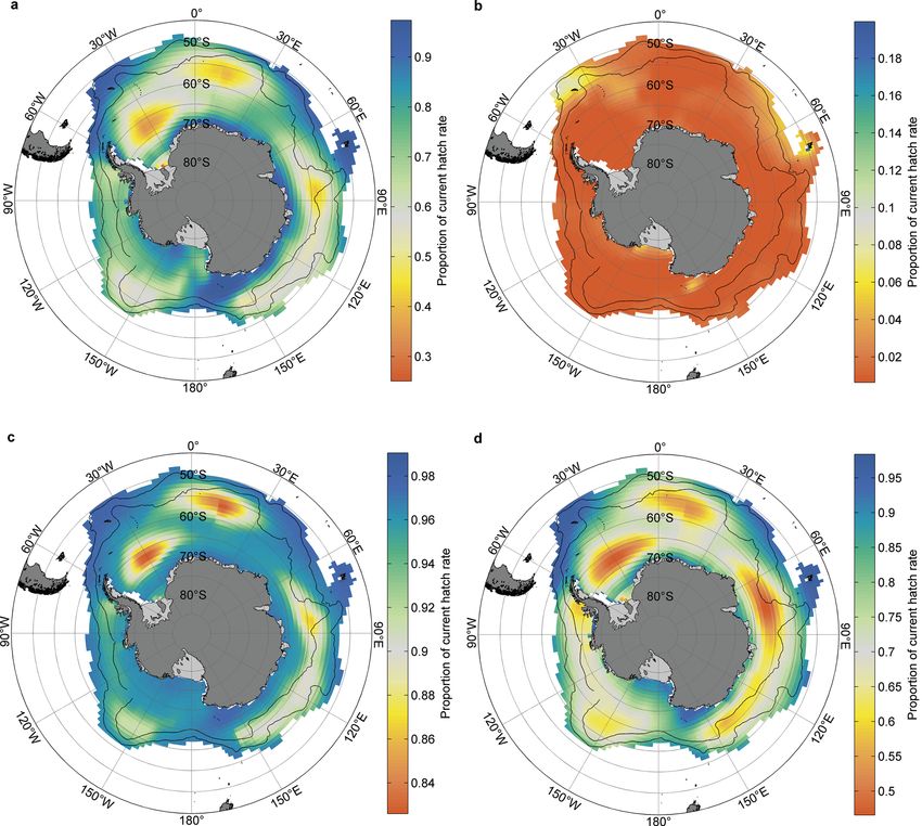
4.3. Growing competition from salps
Salps (mainly Salpa thompsoni) tolerate warmer
water than krill and occupy extensive lower-
productivity regions of the Southern Ocean (Foxton
1966, Le Févre et al. 1998, Nicol et al. 2000a, Pakho-
mov et al. 2002). The occurrence of salps is reported to
be increasing in the southern part of their range ap-
proaching the Antarctic continent (Fig. 9) (Atkinson et
al. 2004). These planktonic tunicates are important
components of marine food webs and are major con-
sumers of production at lower trophic levels. While
salps feed efficiently on a wide range of plankton
(Foxton 1956), they may not efficiently transfer that
energy up to higher levels of the food web (Loeb et al.
1997). The consequences of their trophic dynamics and
changes in their abundance and distribution are
likely to have major effects on the pelagic food web Fig. 9. Krill, salps, and their food. (a) Mean (November−
April) chl a concentration, 1997−2003. (b) Mean krill density
and on pelagic−benthic coupling, through the sedi- (6675 stations, 1926−2003). (c) Mean salp density (5030 sta-
mentation of particulate matter (Raskoff et al. 2005). tions, 1926−2003). Log10(no. krill m–2) = 1.2 log10(mg chl a
As obligate filter feeders, salps tend to prefer m–3) + 0.83 (R2 = 0.051, p = 0.017, n = 110 grid cells). Histori-
oceanic regions with lower food concentrations (Le cal mean positions are shown for the PF29, Southern ACC
Front (SACCF)30, SB30 and northern 15% sea-ice concentra-
Févre et al. 1998, Pakhomov et al. 2002). Thus, lower tions in February and September (1979−2004 means). PF:
productivity across most of the ACC means that suit- Polar Front; SB: Southern Boundary. (Source: figure and de-
able habitat for salps is much larger than for krill scription used with permission from Atkinson et al. 2004)You can also read