Standard Initial Margin Model Seminar @ UNCC - A Practitioner's Perspective

Standard Initial Margin Model Seminar @ UNCC
- A Practitioner’s Perspective
November 22, 2019

Jonathan Wu
Managing Director
Area Head of MRO – Rates, XVA, & FCM
Wells Fargo Bank

Topics

I. Background 3 XII. Benchmarking & Back-testing 45
II. Scope 9 XV. Q & A 48
III. SIMM Implementation Framework 11 XVI. References 49
IV. AcadiaSoft 12
V. Schedule IM 15
VI. Mean and Variance of Portfolio 22
VII. Zero, Forward and Par Rates 25
VIII. SIMM Model 29
IX. SIMM – Interest Rates 32 Disclaimer: The material presented in this deck does not
 contain any company specific information. All examples
X. Curious Case of Interest Rate Vega 37 and numeric analyses used within are public information
 for illustration purpose only. The content is intended for
XI. SIMM – Cross Currency Swap 42 educational and knowledge sharing purpose only.

 2

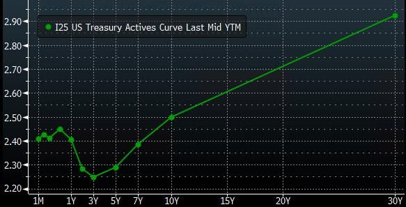
I. Background – Uncleared Margin Rule
– Below is an oversimplified chart showing the regulatory regime changes in responses to
 the financial crises.
– CVA reserve, central clearing, and uncleared margin rule are all measures the institutions
 can take to mitigate the counterparty risk.

 3

I. Background – Capital vs. Margin
– The financial crisis in 2008 raised concerns about the lack of transparency in the over-the-counter
 (OTC) derivatives market and the resiliency of its market participants. To reduce the systemic risk,
 global regulators have made the following important changes:
  Promote Central Clearing – Mandatory Clearing of single currency swaps & CDS in 2013
  Increase the margining amongst the counterparties (include IM & VM)
  Increase the capital buffer
– Both capital and margin perform important and complementary risk mitigation functions but are
 distinct in a number of ways [1].
– Existing capital rules ensure sufficient levels of reserves to act as a buffer in the event of a
 counterparty default. The intent of margin rules is to harmonize “survivor-pay” capital
 requirements with “defaulter-pay” margin rules in order to achieve two regulatory goals:
  Reduce systemic risk in the derivatives market highlighted by the financial crisis, and
  Promote central clearing by aligning bilateral margining with the heightened risk observed in
 bilateral markets.

 Survivor - Pay Defaulter - Pay

 Capital Margin

 4

I. Background – ISDA SIMM
– To level the playing field for the OTC bilateral derivative market from the margin perspective, the Group of 20
 (G20), Basel Committee of Banking Supervision (BCBS), and the International Organization of Securities
 Commissions (IOSCO) created the Working Group on Margin Requirements (WGMR) with the goal of
 establishing a global framework for margin practices of non-cleared over-the-counter derivatives (i.e., bilateral).
– In September 2013, a final policy framework was published by WGMR imposing margin requirements; and global
 regulatory agencies have since developed local rules that are consistent with the WGMR’s framework. This
 framework establishes two-way (i.e., post and collect) initial margin (IM) for certain covered counterparties and
 exchange of variation margin (VM) for covered counterparties. It also restricts the forms of eligible collateral to
 cash and other highly liquid assets, requires mandatory segregation of IM, and requires documentation to govern
 collateral relationships with a bank’s counterparties.
– In December 2013, in order to mitigate differences in IM that banks would calculate by using unique internally
 developed risk-based models, ISDA proposed an initiative to develop a standardized model for computing IM
 that would be compliant with the WGMR policy framework and be utilized by industry participants to collect and
 post IM in accordance with various global margin regimes, including margin rules issued by U.S. prudential
 regulators.
– Over the course of the 4 years since 2013, ISDA incrementally built out the current Standard Initial Margin
 specification, publically available from its website, with a large industry working group. Currently the ISDA SIMM
 is the industry standard and adopted by every in scope SIMM counterparties. ISDA’s success in SIMM
 specification is really rooted on the following 9 objectives it set out to accomplish [2].

 Non-procyclicality Ease of Replication Transparency

 Quick To Calculate Extensible Predictability

 Costs Governance Margin Appropriateness

 5

I. Background - Global Compliance Date
 Initial Margin Starting September 1, 2016 - September 1, 2021 Phase-in metric for IM:
 ► Revised requirement –
 Exceeds Based on aggregate
 VM average notional
 Exceeds
 €3T amounts for March, April,
 Exceeds and May of a given year
 € 2.25T Exceeds when transacting with
 Exceeds another covered entity
 €1.5T (provided that it also
 €0.75T meets that condition).
 €50B
 €8B

 Sep 1, 2016 Mar 1, 2017 Sep 1, 2017 Sep 1, 2018 Sep 1, 2019 Sep 1, 2020 Sep 1, 2020

 Threshold USPR ESAs JFSA
 MTA $500 K € 500 K ¥70 M

 IM Threshold $50 M € 50 M ¥7 B

The threshold value can be different across jurisdictions on the same compliance dates, see the table below:

Country Sep 1, 2016 Sep 1, 2017 Sep 1, 2018 Sep 1, 2019 Sep 1, 2020 Sep 1, 2021

 IM: $3.0T $2.25T $1.5T $0.75T $50B $8B

 IM: €3.0T €2.25T €1.5T €0.75T €50B €8B

 IM: ¥ 420T ¥ 315T ¥ 210T ¥ 105T ¥ 10T? ¥ 1.1T

 6

I. Background – Bilateral Variation Margin

 Counterparty A Counterparty B

– Unidirectional posting
– Generally cash in the same currency as the derivative contract
– Generally can be re-hypothecated
– Netting against the IM not allowed
– Usually called daily but can be called intra-day during volatile market
– Reflecting the MTM of the netting sets.
– Usually you are concerned with two numbers:
  Self calculated MTM
  Counterparty calculated MTM

 7

I. Background – Bilateral Initial Margin

 Counterparty A Custodian Counterparty B

 – Bidirectional posting to a 3rd party custodian
 – Usually non-cash securities subject to the mutually accepted haircut schedule
 – Generally can not be re-hypothecated
 – Netting against the VM not allowed
 – Usually called daily
 – Reflecting the tail risk of the netting sets
 – Intended to cover potential losses in the event of the counterparty defaults
 – Usually you are concerned with four numbers:
  Self calculated Margin to Post (Own Pledgor Amount)
  Self calculated Margin to Collect (Own Secured Amount)
  Counterparty calculated Margin to Post (Counterparty Pledgor Amount)
  Counterparty calculated Margin to Collect (Counterparty Secured Amount)

 8

II. SIMM Scope - Counterparties
– Below are SIMM in scope counterparties for the first 4 waves.
– The in scope company is required to collect IM from its inter-affiliates.

 9

II. SIMM Scope – Product Types
– The Initial Margin rule impacts most of the un-cleared derivative transactions in
 Rates, FX, Equity, Commodities and Credit against all counterparties phased in
 according to the UMR compliance schedule.
– BCBS exempts the physically settled FX forward and swaps for the Margin Rule.
 As the known principle exchanges for a cross currency swap is economically
 equivalent to the FX Forward \ Swaps, all known principle exchanges for cross
 currency swaps are exempted as well.

 Example Product Scope
 Rates FX Commodities Equities Credit
 Cap Non deliverable Forward Commodity Equity Swap CDS ABS Index
 Cancellable Swap Window Forwards Commodity Option Cliquet CDS Index
 Cross Currency Swap FX Option Commodity Swap Variance Swap CDS Structuews Prod
 Digital Cap Com Swaption TRS CDX Index Option
 Digital Floor Power CDS
 Floor Swap Risk Partici. Swap
 Forward Starting Swap TRS
 Inflation Cap
 Inflation Floor
 Inflation Swap
 Swap
 Swaption
 Treasury Lock

 10

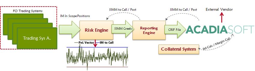
III. SIMM Implementation - Typical High Level Architecture
– Below is a high level system diagram how the SIMM solution could be
 implemented by an in scope company:
  FO Trading Systemswould produce the SIMM specific Greeks as well as other
 position level static attributes including Notinoal
  FO Trading Systems are also responsible for accurately tagging the in scope
 trades for sensitivity calculations (in scope SIMM flag)
  Risk Engine functions as the SIMM sensitivity processing / aggregation engine.
  A Common Risk Interface File (CRIF) is produced by Reporting Engine and
 uploaded to AcadiaSoft [9]
  AcadiaSoft produces the SIMM / Schedule IM numbers and provides a common
 hub for exposure sharing and margin reconciliations.

 11

IV. AcadiaSoft – the Company

- AcadiaSoft, Inc. is the leading industry provider
 of risk and collateral management services for
 the non-cleared derivatives community.
- Owned and backed by the investment of 17
 major industry participants and
 infrastructures, the AcadiaSoft community has
 grown to more than 650 client firms
 exchanging approximately $400B of collateral
 on daily basis.
- Based in Township of Norwell, MA
- {Q} How many Employees of the company?
 • Population of Norwell: 10,506
 • Number of employees: 50 - 200

 12

IV. AcadiaSoft – Calculation Overview
- If AcadiaSoft is used for IM margin hub, SIMM-sensitivities are submitted to AcadiaSoft via Common
 Risk Input File (CRIF) [9].
- The CRIF files are produced and submitted to the vendor at T + 0.
- AcadiaSoft’s IM Exposure Manager provides tools for counterparty reconciliation and investigation of
 IM calculation differences among counterparties as required by UMR regulations and ISDA
 documentation.

 - Trade level sensitivities are calculated by
 participating firms and submitted to
 AcadiaSoft Risk Data Manager

 - AcadiaSoft nets trade level sensitivities and
 aggregates by Bucket, Sensitivity Type, Risk
 Class, Silo, Model and Total.

 - The same process is used to calculate two
 different calculation trees:
 • Pledgor (you pay)
 • Secured Party (you receive)

 - For portfolios containing primarily linear
 products, IM secured will approximate IM
 pledger. Introduction of optionality can cause
 IM pledger and IM secured to diverge
 dramatically.

 13

IV. AcadiaSoft – IM Exposure Manager

 14

IV. Schedule IM
– Schedule IM can be thought as the simplified notional based IM exposure calculation approach.
– It can be a proper approach for smaller firms especially phase 4 or 5 companies to become
 compliant with the UMR without outlandish infrastructure investments.

– Consider the above schedule, we had a long discussion in the initial implementation phase on
 should we classify the Risk Participation Swap as interest rate instrument or credit instrument.
 {Q} Why?
– {Q} Can you think of a situation a bank would rather use the schedule IM as opposed to the
 SIMM modeling approach?

 15

V. Schedule IM
– Consider below live trade for example:

 – {Q} What’s the schedule IM?
 – {Q}How much is produced by AcadiaSoft?

 16

V. Schedule IM
– Consider another live trade for example:

 – {Q} What’s the schedule IM?
 – {Q} How much is produced by AcadiaSoft?

 17

V. Schedule IM
 –{Q} Any potential problems?
  Lack of netting benefit
  Overly punitive
 o A comparative study done by AcadiaSoft for a diversified portfolio could
 produce 7x schedule IM vs. SIMM model. [3]
  Challenge of calculating notional for certain types of derivatives
 o Step up structures
 o Balance guarantee structures
 o Accreting
 o Amortizing
  Tenor classification can also present practical difficulties
 o Callable
 o Extensible

 18

V. Schedule IM – Net to gross ratio
 – In order to address the “lack of the netting benefit” issue, the BCBS
 introduced a workaround – net to gross ratio (NGR). [1]
 – NGR aimes to adjust the Gross Initial Margin Amount in the legally
 enforceable netting set. {Q} Why legal enforceability so important ?

 19

V. Schedule IM – Net to gross ratio
– Without the legal enforceability, a financial institution’s current credit
 exposure to the counterparty equals to its gross positive MTM. [4]
– During the close out if the netting is not legally enforceable, you still
 need to pay your counterparty negative MTM while trying to recover
 your positive MTM.
 Pay $2.2MM
 Rec $4.1MM
 Bank X
 Net Receipt of $1.9MM

 Pay $2.2MM

 Bank X
 Recovery

V. Schedule IM – Net to gross ratio
 – BCBS recognizes the important non-negligible offsets would have been
 ignored if the gross schedule IM were to be implemented without
 considering the netting benefit.
 – BCBS proposes the following formula for calculating the schedule IM by
 taking into the consideration of net to gross ratio (NGR) [1].

 = 0.4 × + 0.6 × × 
 – NGR is defined as the level of the net replacement cost over the level of
 the gross replacement cost for all in scope transactions in the legally
 enforceable netting set.
 – Adjust 60% of Gross IM by NGR.
 – {Q} What’s NGR from Wells Fargo point of view ?
 – {Q} What’s NGR from Bank X point of view?
 Counterparty Net Cost Gross Cost Ratio
 Wells Fargo - 2,173,039.49 0%
 Bank X 1,924,086.50 4,097,125.99 47%

 21

VI. Mean and Variance of Portfolio Return
 – ISDA SIMM model is developed with the shortcomings of the schedule
 IM in mind. It has achieved the universal acceptance in as short as 2.5
 years. There’s no other viable SIMM model outside the ISDA one.
 – The key design principle of the ISDA SIMM is rooted in the classic
 portfolio return and variance theory.
 – Memory refresher 1: {Q} what’s the portfolio return assuming the
 portfolio comprises two assets returning r(1) and r(2) and with w(1) and
 w(2) weighting?
 – Memory refresher 2: {Q} what’s the portfolio variance assuming the
 portfolio comprises two assets having standard deviation of return σ(1)
 and σ(2) and with w(1) and w(2) weighting?

 = 1 × 1 + 2 × 2

 = 12 × σ12 + 22 × σ22 + 2 × 1 × 2 × × 1 × 2

 22

VI. Mean and Variance of Portfolio Return
 – More importantly in general
  Assume we have a portfolio with n assets each return r(i)
  Each asset has a standard deviation of σ (i)
  And the weighting of each asset is w(i)
 – The following define the expected return and the variance of the
 portfolio [5].

 = ෍ × 
 =1

 = ෍ 2 × 2 + ෍ ෍ × × , × × 
 =1 =1 ≠ 

 23

VI. Mean and Variance of Portfolio Return - example
 – Assume we have a portfolio with 2 equal investments in Walmart &
 Target.
 – Walmart returns 3% and Target returns 2%.
 – Walmart’s standard deviation of return is 9% while Target is 7%.
 – The correlation of the returns is 80%.
 – {Q} What’s the portfolio return and risk?

 24

VII. Zero, Forward, and Par Rates
 – It’s very important for us to understand the differences between 3 most
 important rates we work with from time to time:

  Zero Rate: The interest rate that would be earned on a bond that
 provides no coupons [6]. This rate is the point estimate of the yield of
 the instrument at maturity time t and has sufficient information to
 calculate the base NPV of the instrument.

  Forward Rate: Rate of interest for a period of time in the future
 implied by today’s zero rate [6]. E.g., risk driver
 IR_RATE_VAR_USD_LIBSWPM03CME_FWD_BASE_Y05_Y10 has a value
 of 0.027851418 at EOD 4/23, {Q} what does it really mean?

  Par Rate: The coupon (fixed rate) on the bond (vanilla fix – float swap)
 that makes its price (MTM) equal to the principle (zero).

 25

VII. Zero, Forward, and Par Rates
 – Zero Rate: The interest rate that would be earned on a bond that
 provides no coupons [6]. This rate is the point estimate of the yield of the
 instrument at maturity time t and has sufficient information to
 calculate the base NPV of the instrument.

 – The T-bill on the left is trading at
 discount of 2.32375 implying a
 market price of 97.67625.
 – The yield of this bond using simple
 interest is 2.379% while the continual
 compounded yield is approximately
 2.35%.

 100
 = 100 × 
 97.67625
 Source: Bloomberg

 26

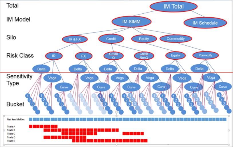
VII. Zero, Forward, and Par Rates
 – Forward Rate: Rate of interest for a period of time in the future implied
 by today’s zero rate [6]
 2 2 − 1 1 1
 = = −1
 2 − 1 2
 – If you know the zero rate at the beginning and the end of the future period, you can easily
 derive the forward rate.
 – The forecast curve in the trading system such as the LIBOR 3M, LIBOR 1M, EURIOR 3M, and
 EURIBOR 6M, contains such information so the expected future cash flows on a derivative
 contracts can be easily computed.
 – {Q} How much is forward rate between December 18, 2019 and March 18, 2010?

 0.98260667 360
 ( 18 2019, 18 2020) = −1 × = 0.025567396
 0.97629699 91

 27

VII. Zero, Forward, and Par Rates
 – Par Rate: The coupon (fixed rate) on the bond (fixed – float swap) that
 makes its price (MTM) equal to the principle (zero).

 – Assuming you want to auction a precise par bond with 2 year maturity.
 {Q} How do you determine the par coupon?
 −0.02448×0.5 −0.02404×1 −0.02348×1.5 
 100 = + + + + 100 −0.02283×2
 2 2 2 2
 = 2.298%

 28

VIII. SIMM Model
 – SIMM uses sensitivities as inputs. Risk factors and sensitivities are clearly
 defined by ISDA and consistently used by all counterparties [7].
 – SIMM sensitivities are used as inputs to aggregation formulae which are
 intended to recognize:
  Hedging
  Diversification benefits
 – SIMM sensitivities are coupled with the “Risk Weights” and aggregated
 with each other using “Correlation Matrices”
 – There are 6 risk classes
 Credit Non-
 Interest Rates Equity FX Commodity Credit Qualifying
 Qualifying

 – There are 4 resultant margin outputs for each of the 6 risk classes
 described above.

 = + + +

 29

VIII. SIMM Model
– There are 4 product classes.
 Rates FX Equity Commodities Credit

– The total margin for that product class is aggregated for its containing risk
 classes.

 = ෍ 2 + ෍ ෍ ψ 
 ≠ 

– The total SIMM is the sum of the above defined product classes.

 SIMM = + + + 

– Please note there’s no diversification benefits across product classes.

 30

VIII. SIMM Model – Aggregate Across Risk Classes
 Credit Non-
 Interest Rates Equity FX Commodity Credit Qualifying
 Qualifying

– Assume your IR risk class pledgor IM = -12,227,022 and FX risk class
 pledger IM = -2,879,051. IR and FX has ψ , = 26%. {Q} How much is the
 SIMM for RatesFX product class?
 = ෍ 2 + ෍ ෍ ψ 
 ≠ 

 = 122270222 + 28790512 + 2 × 0.26 × 12227022 × 287905 = 13270048

 31

IX. SIMM – Delta Margin for Interest Rate
 = + + 
– Following steps are used to calculate the delta margin for interest rates

 1. Obtain weighted sensitivities on par rate IR01 for each index i and tenor k at net level
 Tenor Regular Low-Vol Hi-Vol Ccy Type Ordinal Concentration Type Concentration Threshold
 2w 114 33 91 AUD Regular 2Regular - 28,000,000
 1m 115 20 91 CAD Regular 2Regular - 28,000,000
 3m 102 10 95 CHF Regular 2Regular - 28,000,000
 6m 71 11 88 CNH Hi-Vol 4Hi-Vol 8,000,000
 1y 61 14 99 CNY Hi-Vol 4Hi-Vol 8,000,000
 2y 52 20 101 EUR Regular 2Regular + 230,000,000
 3y 50 22 101 GBP Regular 2Regular + 230,000,000
 5y 51 20 99 HKD Regular 2Regular - 28,000,000
 10y 51 20 108 INR Hi-Vol 4Hi-Vol 8,000,000
 15y 51 21 100 JPY Lo-Vol 3Lo-Vol 82,000,000
 20y 54 23 101 KRW Regular 2Regular - 28,000,000
 30y 62 27 101 MXN Hi-Vol 4Hi-Vol 8,000,000
 NOK Regular 2Regular - 28,000,000
 NZD Regular 2Regular - 28,000,000
 PEN Hi-Vol 4Hi-Vol 8,000,000
 , = × , × PLN Hi-Vol 4Hi-Vol 8,000,000
 SEK Regular 2Regular - 28,000,000
 SGD Regular 2Regular - 28,000,000
 TRY Hi-Vol 4Hi-Vol 8,000,000
 , is the par rate dv01 for index i at tenor k. TWD Regular 2Regular - 28,000,000
 Example: USD 3mL 10yr par rate dv01 USD Regular 2Regular + 230,000,000
 ZAR Hi-Vol 4Hi-Vol 8,000,000

 32

IX. SIMM – Delta Margin for Interest Rate
 = + + 

 2. Obtain delta margins for each currency by aggregating weighted sensitivities across indices
 and tenors within each currency via specified correlations

 2
 ෍ , 
 = + ෍ ෍ φ , ρ , , , 
 , , ( , )≠( , )

 T/T 2w 1m 3m 6m 1y 2y 3y 5y 10y 15y 20y 30y
 % is the correlation b/w any 2 sub- 2w 0.00 0.63 0.59 0.47 0.31 0.22 0.18 0.14 0.09 0.06 0.04 0.05
 curves intra-Ccy, e.g, USD 3mL vs. 1mL
 1m 0.63 0.00 0.79 0.67 0.52 0.42 0.37 0.30 0.23 0.18 0.15 0.13
 3m 0.59 0.79 0.00 0.84 0.68 0.56 0.50 0.42 0.32 0.26 0.24 0.21
 6m 0.47 0.67 0.84 0.00 0.86 0.76 0.69 0.60 0.48 0.42 0.38 0.33
 1y 0.31 0.52 0.68 0.86 0.00 0.94 0.89 0.80 0.67 0.60 0.57 0.53
 2y 0.22 0.42 0.56 0.76 0.94 0.00 0.98 0.91 0.79 0.73 0.70 0.66
 3y 0.18 0.37 0.50 0.69 0.89 0.98 0.00 0.96 0.87 0.81 0.78 0.74
 5y 0.14 0.30 0.42 0.60 0.80 0.91 0.96 0.00 0.95 0.91 0.88 0.84
 10y 0.09 0.23 0.32 0.48 0.67 0.79 0.87 0.95 0.00 0.98 0.97 0.94
 15y 0.06 0.18 0.26 0.42 0.60 0.73 0.81 0.91 0.98 0.00 0.99 0.97
 20y 0.04 0.15 0.24 0.38 0.57 0.70 0.78 0.88 0.97 0.99 0.00 0.99
 30y 0.05 0.13 0.21 0.33 0.53 0.66 0.74 0.84 0.94 0.97 0.99 0.00

 33

IX. SIMM – Delta Margin for Interest Rate
 = + + 

 {Q} Assume we have a positive weighted sensitivity for 2y of 100K and a negative
 weighted sensitivity of 3yr of -100K all on 3mL; what’s our IM?

 2
 = ෍ , + ෍ ෍ φ , ρ , , , 
 , , ( , )≠( , )

 % between 2 sub-curves intra-Ccy, % is the correlation b/w 2yr and 3yr
 e.g, 3mL vs. 1mL, 100% if same curve par rate sensitivities

 = 1002 + −100 2 + 100% × 98% × 100 × −100 × 2 = 2 × 100 × (100 − 98) = 20 

 {Q} Assume we have a positive weighted sensitivity for 2y of 100K on 3mL
 and a negative weighted sensitivity of 3yr of -100K on 1mL; what’s our IM?

 = 1002 + −100 2 + 98% × 98% × 100 × −100 × 2 = 2 × (1002 −982) = 2 × 198 = 28.14 

 34

IX. SIMM Model – Delta Margin for Interest Rate
 = + + 

 3. Obtain delta margin by aggregate across currencies with specified correlations

 = ෍ 2 + ෍ ෍ , , Accounting for risk offset cross currencies but
 limited by the correlation
 ≠ 

 21% should be used for aggregating = max(min(෍ , , ), − )
 across different currencies.
 , 

 is always non-negative
 − is always non-positive
 , Could be positive or negative or zero
 preserves the signage of the exposure,
 hence ensuring the netting benefit

 35

IX. SIMM Model – Delta Margin for Interest Rate
 = + + 

 {Q} Assume we have a short USD 3yr 3mL PV01 =2K and a long EUR 3yr 3mE -2K; what’s
 our IM?

 = ෍ 2 + ෍ ෍ , , = max(min(෍ , , ), − )
 ≠ , 

 21% should be used for aggregating is always non-negative
 across different currencies. − is always non-positive
 , Could be positive or negative or zero
 preserves the signage of the exposure,
 hence ensuring the netting benefit

 = 2 × 50 = 100 ; = −2 × 50 = −100 

 = 100 ; = −100 
 = 1002 + −100 2 + 2 × 21% × 1 × 100 × (−100) = 2 × 100 × (100 − 21) = 125.69 

 36

X. SIMM – Curious Case of Interest Rate Vega
 = + + 

 Vega for the corresponding
 = ෍ 
 vol grid point
 
 Implied volatility for
 tenor k and expiry j

– Interesting to see ISDA spec requires the implied volatility level to be
 used as the operand to multiply with the vega. Why ?
– AcadiaSoft requires the submission of vega risk to be the product of
 vega and the ATM Vol as well.
– It turns out it solves the vega risk representation issue elegantly.
 Different banks may have implemented different vega risk metrics.
 Some may produce black (a.k.a. lognormal) vega; some may instead
 produce normal vega.
– By asking for the vega X ATM Vol, ISDA SIMM achieves the vega risk
 submission invariance. {Q} Why this will give us vega risk invariance?

 37

X. SIMM – Curious Case of Interest Rate Vega
 = + + 

 Vega for the corresponding
 = ෍ 
 vol grid point
 
 Implied volatility for
 tenor k and expiry j

– To see this mathematically (black vega x black vol ≃ normal vega x normal vol)

 = × 
 
 = 
 
 × = × × σ 
 
 × = × × 
 
 × = × 
 
 38

X. SIMM – Curious Case of Interest Rate Vega
 = + + 

 = ෍ 
 
– Is it empirically true ?
 Type ATM Vol Vega Product

 Black 23.13 262,824.40 6,079,128.37

 Normal 56.99 69,927.18 3,985,149.99

– Appears to be very different
 for the 1y10y ATM swaption
– {Q} Why?

 39

X. SIMM – Curious Case of Interest Rate Vega
 = + + 

 – This turns out partially explainable due to our shifted SABR model.
 – We pushes up the forward rates by 125bps which impacts the black vega # and ATM log
 normal volatility.

 – If you use our internal shifted SABR produced lognormal volatility, you can see the vega
 invariance roughly holds:
 black vega x black vol ≃ normal vega x normal vol
 1y10y ATM Vol Vega Product
 Black 15.15 (262,824) (3,981,790)
 Normal 56.99 (69,927) (3,985,150)

 40

X. SIMM – Curious Case of Interest Rate Vega
 = + + 

– The industry model validation on ISDA SIMM reported an issue on the
 “Invariance” of vega sensitivity under normal vs. lognormal.
 
 = 1 −
 24
– The model validation concluded “As the time to maturity becomes longer,
 this approximation deviates more significantly” [8].
 10y10y ATM Vol Vega Product
 Black 14.12 (707,464) (9,989,390)
 Normal 57.84 (175,422) (10,146,403)
 Diff (157,013)
 % Diff 1.55%
 1y10y ATM Vol Vega Product
 Black 15.15 (262,824) (3,981,790)
 Normal 56.99 (69,927) (3,985,150)
 Diff (3,360)
 % Diff 0.08%
 3m10y ATM Vol Vega Product
 Black 13.68 (132,557) (1,813,378)
 Normal 51.86 (35,409) (1,836,300)
 Diff (22,922)
 % Diff 1.25%
 41

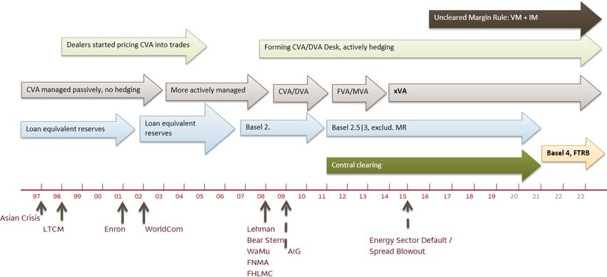
XI. SIMM – Cross Currency Swaps
– SIMM treatment on Cross Currency Swaps
 ushered in controversial feedbacks. $500MM €442MM
 x x
– Due to Basel Rule explicitly exempt FX forward Principal Principal
 and swaps for the Initial Margin Rule [1], the
 physical principal exchanges which are
 economically equivalent to FX forward and
 swaps are also excluded [1, 7]. 3mL 3mE – 20BP
– All fixed notional cross currency swaps’
 principle exchanges are excluded [10]
  Constant Notional
  Amortizing
  Accreting
– Notional resettable cross currency swaps $500MM €442MM
 x
 x Principal Principal
  Only the principle changes associated with
 the current period can be ignored for margin
 calculation [10].

 42

XI. SIMM – Cross Currency Swaps
 FX Delta
 IR Delta

 Delta Margin

 Risk Weight

 43
 XCCy Basis

FX Delta
XI. SIMM – Cross Currency Swaps

 IR Delta

 Delta Margin

 Risk Weight

 XCCy Basis
 44

XII. SIMM – Benchmarking & Back-testing
– U.S. and European final rules require monitoring and assessment of controls,
 validation and operational process and procedures surrounding margin model [11].
– Regulators require ongoing portfolio level SIMM monitoring for IM sufficiency thru
 benchmarking and back-testing[11]. The back-testing results are to be shared with the
 ISDA on quarterly basis.
– The idea is to identify if we have IM shortfalls based on the current in force SIMM
 methodology using the classic back-testing tool. Statistically the portfolio level
 monitoring seeks to verify the secured (pledgor) IM based on the SIMM methodology
 ensures the firm (counterparty) will not suffer losses for a 10-day horizon at 99%
 confidence level.
– Conducting the back-testing at netting set level at the regular interval is an onerous
 exercise. We have some relief that it’s technically not required on the portfolios with
 SIMM margin < €50MM.
– The firms are expected to report to ISDA the margin coverage shortfalls.
– Unidirectional monitoring is allowable to reduce the burden on the smaller firms.

 WFC

 45

XII. SIMM – Benchmarking & Back-testing
– SIMM shortfall amount is defined as the “smallest incremental margin amount
 that would give Green Traffic light signal from a back-testing using the 99%
 confidence level” [11].
  1+3 back-testing
  Comparison of actual portfolio “1-day Clean P&L” vs. “1-day SIMM”

 46

XII. SIMM – Benchmarking & Back-testing
– The number of exceedances in “1+3” period is categorized in “Red”, “Amber” and
 “Green” zone based on modified Basel traffic light approach [12]. Below is an
 illustration of how the threshold will look like assuming 1000 observations.

 > 44 Exceedances

 > 21 Exceedances but

XV. Question & Answers
– If there are follow up questions, please email: jonathan.wu@wellsfargo.com

 48

XVI. References
 [1] BCBS & IOSCO: Margin Requirements for Non-Centrally Cleared Derivatives, March
 2015. url: https://www.bis.org/bcbs/publ/d317.pdf
 [2] ISDA: Standard Initial Margin Model for Non-Cleared Derivatives. December 2013. url:
 https://www.isda.org/a/mMiDE/simm-for-non-cleared-20131210.pdf
 [3] AcadiaSoft: A Comparative Analysis of Initial Margin Models. 2018. url:
 https://www.acadiasoft.com/wp-content/uploads/2018/08/SIMMvsSCHEDULE_2018.pdf
 [4] ISDA: Netting and Offsetting: Reporting derivatives under US GAAP and under IFRS.
 May 2012. url: https://www.isda.org/a/veiDE/offsetting-under-us-gaap-and-ifrs-may-
 2012.pdf
 [5] Simon Benninga: Financial Modeling, 3rd Edition. MIT Press 2008
 [6] John Hull: Options, Futures, and Other Derivatives. 6th Edition. Prentice Hall 2009
 [7] ISDA: SIMMTM Methodology version 2.1. December 2018. url:
 https://www.isda.org/a/zSpEE/ISDA-SIMM-v2.1-PUBLIC.pdf
 [8] ISDA: ISDA SIMM Model Validation Report. October 2015.
 [9] ISDA: SIDA SIMM Methodology: Risk Data Standards. February 2017
 [10] Wells Fargo FX Quants: FIX 207: FX Market Risk Bumping Methodology. 2017
 [11] ISDA: ISDA SIMM Governance Framework. September 2017. url:
 https://www.isda.org/a/7FiDE/isda-simm-governance-framework-19-september-2017-
 public.pdf

 49