Sudden Stratospheric Warmings - Ed Gerber

REVIEW ARTICLE Sudden Stratospheric Warmings
10.1029/2020RG000708
 Mark P. Baldwin1 , Blanca Ayarzagüena2 , Thomas Birner3,4 , Neal Butchart5 ,
Key Points: Amy H. Butler6 , Andrew J. Charlton-Perez7 , Daniela I. V. Domeisen8 ,
• Sudden stratospheric warmings
 are dramatic events of the polar Chaim I. Garfinkel9 , Hella Garny4 , Edwin P. Gerber10 , Michaela I. Hegglin7 ,
 stratosphere that affect the Ulrike Langematz11 , and Nicholas M. Pedatella12,13
 atmosphere from the surface to the
 thermosphere 1 Global Systems Institute and Department of Mathematics, University of Exeter, Exeter, UK, 2 Dpto. de Física de la
• Our understanding of sudden
 Tierra y Astrofísica, Facultad de CC. Físicas, Universidad Complutense de Madrid, Madrid, Spain, 3 Meteorological
 stratospheric warmings has
 accelerated recently, particularly Institute, Ludwig Maximilian University of Munich, Munich, Germany, 4 Deutsches Zentrum für Luft- und Raumfahrt
 the predictability of surface weather (DLR), Institut für Physik der Atmosphäre, Oberpfaffenhofen, Germany, 5 Met Office Hadley Centre, Exeter, UK,
 effects 6 NOAA Chemical Sciences Laboratory, Boulder, CO, USA, 7 Department of Meteorology, University of Reading,
• More observations, improved Reading, UK, 8 Institute for Atmospheric and Climate Science, ETH Zurich, Zurich, Switzerland, 9 The Fredy & Nadine
 climate models, and big data
 Herrmann Institute of Earth Sciences, The Hebrew University, Jerusalem, Israel, 10 Courant Institute of Mathematical
 methods will address
 uncertainties in key aspects of Sciences, New York University, New York, NY, USA, 11 Institut für Meteorologie, Freie Universität Berlin, Berlin,
 sudden stratospheric warmings Germany, 12 High Altitude Observatory, National Center for Atmospheric Research, Boulder, CO, USA, 13 COSMIC
 Program Office, University Center for Atmospheric Research, Boulder, CO, USA

Correspondence to:
M. P. Baldwin,
m.baldwin@exeter.ac.uk
 Abstract Sudden stratospheric warmings (SSWs) are impressive fluid dynamical events in which large
 and rapid temperature increases in the winter polar stratosphere (∼10–50 km) are associated with a
 complete reversal of the climatological wintertime westerly winds. SSWs are caused by the breaking of
Citation:
Baldwin, M. P., Ayarzagüena, B.,
 planetary-scale waves that propagate upwards from the troposphere. During an SSW, the polar vortex
Birner, T., Butchart, N., Butler, A. H., breaks down, accompanied by rapid descent and warming of air in polar latitudes, mirrored by ascent and
Charlton-Perez, A. J., et al. (2021). cooling above the warming. The rapid warming and descent of the polar air column affect tropospheric
Sudden stratospheric warmings.
Reviews of Geophysics, 59,
 weather, shifting jet streams, storm tracks, and the Northern Annular Mode, making cold air outbreaks
e2020RG000708. https://doi.org/10. over North America and Eurasia more likely. SSWs affect the atmosphere above the stratosphere,
1029/2020RG000708 producing widespread effects on atmospheric chemistry, temperatures, winds, neutral (nonionized)
 particles and electron densities, and electric fields. These effects span both hemispheres. Given their
Received 9 APR 2020 crucial role in the whole atmosphere, SSWs are also seen as a key process to analyze in climate change
Accepted 10 NOV 2020 studies and subseasonal to seasonal prediction. This work reviews the current knowledge on the most
Accepted article online 23 NOV 2020
 important aspects of SSWs, from the historical background to dynamical processes, modeling, chemistry,
 and impact on other atmospheric layers.

 Plain Language Summary The stratosphere is the layer of the atmosphere from ∼10 to
 50 km, with pressures decreasing to ∼1 hPa (0.1% of surface pressure) at the top. The polar stratosphere
 during winter is normally very cold, with strong westerly winds. Roughly every 2 years in the Northern
 Hemisphere, the quiescent vortex suddenly warms over a week or two, and the winds slow dramatically,
 resulting in easterly winds that are more similar to the summer. These events, known as sudden
 stratospheric warmings (SSWs), were discovered in the early 1950s, and today, they are observed in detail
 by satellites. After several decades researching SSWs, considerable progress has been made in dynamical
 aspects of SSWs, but our understanding of how they affect both surface weather and the upper atmosphere
 is incomplete. We observe that variability of the stratospheric circulation (SSWs being an extreme event)
 is associated with shifts in the jet stream and the paths of storms, with associated effects on rainfall and
 temperatures. The likelihood of cold weather spells and damaging wind storms is also affected. Almost
 all SSWs have occurred in the Northern Hemisphere, but there was one spectacular major SSW in 2002 in
 the Southern Hemisphere.

 1. Introduction
 Sudden stratospheric warmings (SSWs) are the most dramatic stratospheric phenomenon. During SSWs,
©2020. American Geophysical Union. the normally strong wintertime westerly stratospheric circulation breaks down in a few days and is replaced
All Rights Reserved. by weak easterly winds. This is accompanied by polar warming by up to 50◦ C; the effects extend to

BALDWIN ET AL. 1 of 37

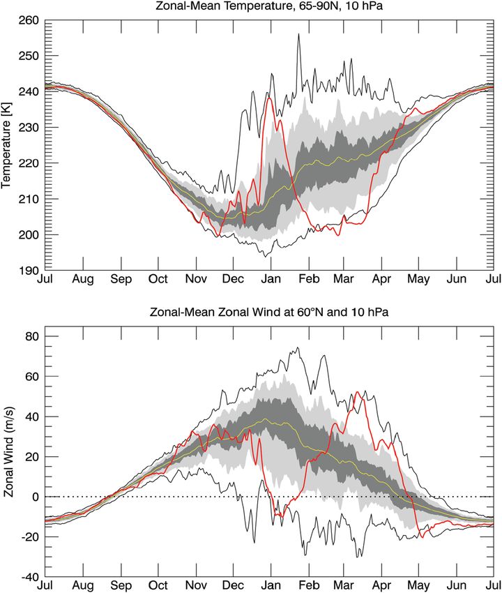
Reviews of Geophysics 10.1029/2020RG000708

 Figure 1. 10-hPa 65–90◦ N ERA-Interim reanalysis (Dee et al., 2011) zonal-mean temperatures (top) and zonal-mean
 zonal wind at 60◦ N (bottom) for July 2018 to June 2019 (red lines). An SSW event is seen as the upward spike in
 temperature and the reduction to less than 0 m/s in zonal wind (easterlies). The yellow lines signify the daily average
 conditions in the stratosphere for that time of year, while the gray shading shows 30th/70th (dark) and 10th/90th
 (light) percentiles. Solid black lines show the daily max/min for prior winters 1979–2018. The month ticks indicate the
 first day of the month.

 Earth's surface as well as through the mesosphere and beyond. The climatology of both the mean flow
 and planetary-scale wave amplitudes determines the overall likelihood of SSWs, which occur only during
 extended winter and almost exclusively in the Northern Hemisphere (NH).
 The variation of insolation with latitude and season drives a strong annual cycle in the stratosphere. Dur-
 ing winter, the polar stratosphere is characterized by a strong, westerly, cold polar vortex. The polar vortex
 is formed primarily through radiative cooling and is characterized by a band of strong westerly winds at
 middle to high latitudes. Typical temperatures are approximately -65◦ to -55◦ C (∼208–218 K) in the polar
 NH at 10 hPa. Roughly every 2 years, the wintertime vortex is disrupted by planetary-scale waves to such
 an extent that this circulation breaks down, with westerly winds becoming weak easterly, and temper-
 atures climbing several tens of ◦ C—essentially summertime conditions—and occasionally (e.g., January
 2009) climbing above 0◦ C at some local points. SSWs happen very rapidly, i.e., in a few days, resulting in
 one of the most dramatic atmospheric events. Figure 1 illustrates a sudden warming event in 2018–2019,
 together with the background climatology and variability of zonal wind, and the average temperature
 from 65◦ N to 90◦ N at 10 hPa. It is important to highlight that both the lowest and highest recorded

BALDWIN ET AL. 2 of 37

Reviews of Geophysics 10.1029/2020RG000708

 temperatures occurred in midwinter. Outside of winter, the stratosphere
 is quiescent. The warming event (red curve) was followed, after more
 than a month, by anomalously low temperatures and strong winds in
 the middle stratosphere. Figure 2 illustrates zonal mean temperature
 anomalies averaged over 0–30 days following SSW events. The upper
 stratosphere cools, and that there is slight cooling in the midlatitudes
 and tropics in compensation for the downward adiabatic warming over
 the polar cap. Vectors illustrate the approximate motion consistent with
 the temperature anomalies (and pressure anomalies, not shown). See
 Baldwin et al. (2019) for details of the calculation. In particular, note the
 poleward movement of mass near the surface at high latitudes. This leads
 to higher Arctic surface pressure following SSWs.
 The effects of SSWs are not only identified in the middle stratosphere.
 SSWs last much longer in the lower stratosphere and troposphere than
 they do in the upper stratosphere. Figure 3a illustrates a lag composite of
 temperature anomalies for SSW events in JRA-55 reanalyses (1958–2015).
Figure 2. Composite temperature anomalies averaged during Days 0–30 Above 30 km, the SSW events end within 2–3 weeks, while in the low-
following 36 SSW events during 1958–2015 in JRA-55 data (1,116-day
mean) (Kobayashi et al., 2015). The SSW dates are defined based on the ermost stratosphere, SSWs last more than 2 months, on average. This is
reversal of the zonal mean zonal wind at 60◦ N and 10 hPa, applying the largely due to the faster radiative time scale in the upper stratosphere.
criterion of Charlton and Polvani (2007). The contour interval is 1 K. The Pressure anomaly composites (Figure 3b) are similar to temperature,
vertical component of the vectors represent the approximate displacement except that surface effects are clearly visible. The “lumpiness” of the sur-
(from the climatological basic state) to form the temperature anomalies
shown. Similarly, the horizontal components represent the north-south
 face signal is due to averaging of a relatively small number of SSWs.
movement consistent with pressure regressions (not shown). The vectors Averaged over 0–60 days, the surface pressure anomaly is 2.1 hPa but is
are derived statistically from regressions and are not a dynamical only 0.74 hPa near the tropopause. This is called “surface amplification”
circulation. Beginning with the basic state, atmospheric movement defined of the stratospheric signal (Baldwin et al., 2019). The fact that the pressure
by the vectors would create temperature and pressure anomalies
 anomaly from SSWs is largest at the surface is important. It means that
approximately equal to the regression values. The calculation was
performed in height coordinates. The pressure labels are approximate. The tropospheric near-surface processes must be reinforcing the stratospheric
lapse-rate tropopause (gray line) is shown for the days in the composite. signal, raising surface pressure over the polar cap (see section 7).
 SSWs are fascinating from a fluid dynamical perspective, and perhaps,
 the simplest and most insightful way of viewing the dynamics is maps of
 potential vorticity (PV; see section 4) (McIntyre & Palmer, 1983, 1984). Maps of PV in the middle stratosphere
 show that planetary-scale wave breaking erodes the polar vortex, sharpening its edge. All SSWs are preceded
 by erosion of the vortex, which forms a “surf zone” surrounding the vortex. With fine enough resolution,
 one can see filamentation—thin streamers—of PV being stripped away from the vortex and mixed into the
 surf zone. This horizontal view complements the zonal mean, which shows mainly rapid temperature rises
 as air descends over the polar cap, accompanied by slowing of the zonal winds. Over time, differing mecha-
 nisms have been suggested to explain the occurrence of SSWs. Some of the mechanisms are complementary
 descriptions from different perspectives, e.g., the zonal-mean perspective of wave, mean-flow interaction,
 vs. the horizontal perspective of wave breaking and PV. These issues are discussed in section 4.
 An underlying question is whether or not SSWs are dynamically unique extreme events. Given the observed
 distributions of temperatures, winds, PV, etc., do SSWs stand out as outliers from the distribution? Or is it
 that SSWs simply occupy one tail of the distribution? In the NH, it appears that SSWs occupy one tail of
 the distribution (e.g., of wintertime of zonal mean wind at 60◦ N, 10 hPa). There is a broad continuum of
 warmings, from very minor to major deviations from climatology (Coughlin & Gray, 2009). Thus, defining an
 SSW as having occurred or not comes down to defining a fixed threshold (e.g., of absolute stratospheric fields
 such as polar wind and/or temperature at some level) or a relative field (e.g., based on the variability of the
 polar stratosphere such as the Northern Annular Mode (NAM) or just the variability of the polar temperature
 Butler et al., 2015). As summarized in section 3, many different criteria have been proposed for detecting
 major SSW events. They often identify the most disruptive events but differ in the quantitative size and
 timing of the events. However, the use of different algorithms in studies can lead to inconsistent conclusions
 among studies, particularly when using different models or under different climate states (McLandress &
 Shepherd, 2009).

BALDWIN ET AL. 3 of 37

Reviews of Geophysics 10.1029/2020RG000708

 Figure 3. (a) Lag-composite of polar cap (65–90◦ N) mean temperature anomalies from 36 SSW events during
 1958–2015 in JRA-55 data. The SSWs dates are defined based on the reversal of the zonal mean zonal wind at 60◦ N and
 10 hPa, applying the criterion of Charlton and Polvani (2007). The contour interval is 1 K. The tropopause (gray line) is
 depressed by ∼750 m following the warmings. (b) as in (a) except for polar cap pressure anomalies. Contour interval
 0.25 hPa

 So far we have mainly focused on the NH, since all major SSWs occurred in the NH prior to 2002. In fact, in
 the Southern Hemisphere (SH), there has been only one major SSW (in 2002), and it was indeed spectacular
 (Krüger et al., 2005). In terms of daily zonal wind anomalies, the event was approximately eight standard
 deviations from the mean—far outside the distribution up to that time. As rare as this event was, in early
 September 2019, a similarly anomalous event occurred, though it did not technically qualify as a major SSW
 by established criteria (Hendon et al., 2019; Rao et al., 2020). SH warming events are important because they
 inhibit strong heterogeneous ozone depletion—essentially preventing the formation of the ozone hole—and
 because these events affect jet streams, precipitation (and droughts) especially across Australia (e.g., Lim
 et al., 2019; Thompson et al., 2005).
 The effects of SSWs are not confined to the polar stratosphere. SSWs affect the circulation in the tropical
 stratosphere (e.g., Kodera et al., 22011) and beyond, mixing chemical constituents such as ozone, as indicated
 in section 9. The large descent over the polar cap associated with the SSW is balanced by upwelling south of
 ∼50◦ N that extends into the SH (Figure 2). Also visible is ascent (cooling) in the polar upper stratosphere,
 that extends into the mesosphere (Körnich & Becker, 2010). SSWs can affect thermospheric chemistry,

BALDWIN ET AL. 4 of 37

Reviews of Geophysics 10.1029/2020RG000708

 temperatures, winds, electron densities, and electric fields, across both hemispheres (Chau et al., 2012).
 These effects are discussed in section 8.
 Some of the most important impacts of SSWs occur in the troposphere, and this is actually one of the SSW
 features that has received most of the attention in literature in the last decade—as summarized in section 7.
 On average, SSWs are observed to have substantial, long-lasting effects on surface weather and climate,
 especially on sea-level pressure (SLP) and the NAM, with associated shifts in the jet streams, storm tracks,
 and precipitation (e.g., Baldwin & Dunkerton, 2001). These effects are much larger than can be explained
 by dynamical theories such as PV inversion (e.g., Charlton et al., 2005) or the tropospheric response to
 stratospheric wave forcing. Tropospheric processes, possibly involving low-level Arctic temperature anoma-
 lies, act to amplify the stratospheric signal (Baldwin et al., 2019). This picture of SSW impacts on surface
 weather becomes clear when analysis over many SSWs is averaged together. Despite the extensive efforts of
 the scientific community, it is still impossible to predict which individual SSW will have a visible downward
 impact—meaning that the tropospheric anomalies (e.g., NAM index or pressure) are of the same sign as as
 those in the stratosphere. Some SSWs may have a tropospheric impact, but not enough to be obvious.
 Given the relevance of SSW events on the whole atmosphere, several efforts have been made in investigat-
 ing their predictability. SSWs can be predicted relatively well 10–15 days in advance (Domeisen et al., 2020a;
 Karpechko, 2018; Tripathi et al., 2015). Several phenomena outside the polar stratosphere have been iden-
 tified, in the observations, as possible modulators of the likelihood of SSWs. Some of them are related to the
 tropical stratosphere such as the quasi-biennial oscillation (QBO) and semiannual oscillation (SAO) of the
 equatorial stratosphere. Others are related to ocean-atmosphere system such as the El Niño-Southern Oscil-
 lation (ENSO) and Madden-Julian Oscillation (MJO), and some others even refer to external phenomena
 such as the 11-year solar cycle. With multiple possible influences, and only around 40 SSWs since 1958,
 quantifying these relationships is challenging.
 In this study, we offer a review of our current understanding of most aspects of SSWs. Most of the previous
 reviews of SSWs were published several decades ago and only or mostly focused on the explanation of the
 dynamics involved in the occurrence of these events (e.g., Holton, 1980; McIntyre, 1982; Schoeberl, 1978).
 Around 1980, the availability of observations in the stratosphere was very limited, mainly because mete-
 orological satellites were just starting to operate. This hindered the investigation of SSW aspects such
 as the effects on the upper atmosphere. Surface weather effects were not widely recognized until 1999
 (e.g., Baldwin & Dunkerton, 1999). Another limitation was that general circulation models (GCMs) in the
 1970s and 1980s had low vertical resolution of the stratosphere. The biggest increase in the number models
 with well-resolved stratospheres was relatively recent, during the Coupled Model Intercomparison Project
 Phase 5 (CMIP5) (Charlton-Perez et al., 2013). Model development has not only allowed the advance in
 knowledge on known dynamical and chemistry aspects but also the exploration of new SSW perspectives
 such as the benefits of including stratospheric information to improve medium range to subseasonal predic-
 tions of surface weather. Research on SSWs has accelerated in very recent decades with a large increase in
 the number of publications on this topic. Summaries have been written by O'Neill et al. (2015) and Padatella
 et al. (2018), but not in detail, or just covering the most common aspects such as dynamics, types of events,
 history, or tropospheric fingerprint. For instance, O'Neill et al. (2015) do not address the effects of SSWs on
 the atmosphere above the stratopause, whereas Padatella et al. (2018) provide just an overview of SSWs influ-
 ence on the whole atmosphere without going much in detail. Still, as anticipated previously, many questions
 remain open. The present review aims to provide a general overview of SSWs by covering the major aspects
 of SSWs, their impacts, and the outstanding research challenges. In section 2, a brief historical background
 is provided, and section 3 describes the classification of these events. Dynamical theories for the occurrence
 of SSWs are included in section 4, and possible external factors driving SSWs are discussed in section 5. The
 predictability of SSWs is discussed in section 6, and their effects on climate and weather are presented in
 section 7. Effects above the stratosphere are described in section 8, and chemical/tracer aspects are shown
 in section 9. Finally, the outlook/conclusion is provided in section 10.

 2. Historical Background
 SSWs were discovered by Richard Scherhag in radiosonde temperature measurements above Berlin,
 Germany. Scherhag started regular radiosonde measurements from the area of the former Tempelhof airport
 in Berlin in January 1951. As professor and head of the recently founded Institute of Meteorology at Freie

BALDWIN ET AL. 5 of 37

Reviews of Geophysics 10.1029/2020RG000708

 Universität Berlin, he was interested in exploring the stratosphere. With
 the help of the U.S. allies in postwar Berlin, he was able to employ a
 new type of American radiosonde using neoprene balloons which pro-
 vided regular measurements of the stratosphere up to ∼30 km altitude
 (∼10 hPa). In a first publication in spring 1952, Scherhag reported an
 explosive-type warming of the high stratosphere in January 1952 and
 concluded that the observed warming was too strong to be explained by
 advection (Scherhag, 1952a). This “Berlin Phenomenon,” as Scherhag
 called the warming, developed as follows: “While all measured strato-
 spheric temperatures ranged between -56◦ C and -69◦ C on 26 January,
 only two days later -37◦ C were measured at 13 hPa. This means a sudden
 warming of 30◦ C had started on 27 January. On 30 January, the temper-
 ature reached -23◦ C in 10 hPa, followed by a rapid cooling.” Scherhag
 also found that the warming slowly propagated downward to the 200-hPa
 pressure level within 1 week. This first warming pulse was followed by
 a second, even stronger warming about 1 month later, with a tempera-
 ture maximum of -12.4◦ C (a warming of ∼37◦ C within 2 days) at 10 hPa
 on 23 February and a change in circulation to southeasterly winds in the
 middle stratosphere. Figure 4 shows the Tempelhof radiosonde temper-
 ature measurements of 21 February (before the warming), 23 February
 (at the peak of the SSW), and 28 February (after the peak) (Wiehler, 1955).
 Also in February 1952, upper level wind data from radiosondes over
 the northern United States indicated an increase of the frequency of
Figure 4. Radiosonde temperature measurements in Berlin-Tempelhof
 easterly winds at 50 hPa associated with a closed persistent anticyclonic
during the first recorded sudden stratospheric warming in 21–28 February circulation northwest of Hudson Bay and a warming over Canada and
1952. Figure from Wiehler (1955). Greenland (Darling, 1953).
 In a first attempt to explain the unexpected warming of the winter stratosphere, Scherhag (1952b) and
 Willett (1952) suspected a severe solar eruption on 24 February to be the source. While we now know that
 solar effects are not strong enough to force individual SSWs, a statistical relation between the occurrence
 of SSWs and solar activity is actively discussed until the present day. A similar stratospheric warming had
 also been noted the year before, in February 1951, from British Meteorological Office radiosonde and radar
 measurements over England and Scotland. It was accompanied by a reversal of the lower stratospheric
 winds to easterlies which were followed again by westerlies before the transition to summertime easterlies
 (Scrase, 1953). It then took until the winters 1956/57 and 1957/58 that similarly strong SSWs were analyzed

Figure 5. 50-hPa temperature time series over Alert, Ellesmere Land, during the three winters with stratospheric warmings in the 1950s. Figure from
Warnecke (1962).

BALDWIN ET AL. 6 of 37

Reviews of Geophysics 10.1029/2020RG000708

Figure 6. 10-hPa height map on 18 January 1963 (left) and 27 January 1963 (middle) and sea-level pressure on 31 January 1963 (right) (Figure from Scherhag
(1965)). ©Springer. Used with permission.

 in maps which had been specifically produced on stratospheric pressure levels (Teweles, 1958; Teweles &
 Finger, 1958). Figure 5 shows the evolution of 50-hPa temperature over Alert, Ellesmere Land, during three
 winters with stratospheric warmings in the 1950s.
 With the start of the International Geophysical Year (IGY) in July 1957, the number of radiosonde bal-
 loons reaching altitudes above 30 km increased. Stratospheric maps (daily or every 5 days, at 100, 50, 30, and
 10 hPa) for the NH were published by several centers, e.g., the U.S. Weather Bureau, the Arctic Meteorology
 Research Group of McGill University Montreal and the Stratospheric Research Group of Freie Universität
 Berlin. Meteorological rocketsondes provided new insights: it was found, for example, that the strong strato-
 spheric warming over Fort Churchill in January 1958 occurred a couple of days earlier in the altitude region
 above 40 km than in the layers below (Stroud et al., 1960). Moreover, intense warmings were detected in
 the upper stratosphere which were never detected below 10 hPa. In order to obtain an increased number of
 high-altitude soundings during stratospheric warmings, the STRATWARM warning system was established
 by the WMO in 1964. These alerts included information on the intensity and movement of the warm-
 ings and were distributed internationally from the meteorological centers at Melbourne, Tokyo, Berlin, and
 Washington D.C. As suggested in the WMO/IQSY (1964) report, SSWs were classified according to their
 time of occurrence (“midwinter warmings” vs. “final warmings” in late winter) and their intensity. While
 “minor midwinter warmings” were characterized by a strong warming of the Arctic stratosphere at 10 hPa
 and higher levels, “major midwinter warmings” had to be additionally accompanied by a complete circula-
 tion reversal from westerlies to easterlies polewards of 60◦ N at the same levels. Alternative SSW definitions
 that were developed later are discussed in section 3.
 In a plea for additional upper air data, Scherhag et al. (1970) raised the question of “whether an intimate
 knowledge of the stratospheric circulation would prove valuable in, for example, forecasting.” They stated
 that phase relationships between events in the stratosphere and troposphere must be known for a full explo-
 ration of forecast probabilities. In fact, Scherhag had speculated about the impact of SSWs on surface weather
 as early as in his initial 1952 report, in which he pointed out a drop in forecast skill score following the
 February 1952 SSW (perhaps related to the fact that stratospheric information was not included in the fore-
 casts). Indeed, some early studies had pointed at a potential interaction of tropospheric and stratospheric
 zonal wavenumber 2 during the 1967/68 warming (Johnson, 1969) and the role of tropospheric blockings for
 the onset of stratospheric warmings (Julian & Labitzke, 1965). An early example of stratosphere-troposphere
 coupling is illustrated in Figure 6 which shows 10-hPa height maps at the beginning (18 January, left panel)
 and peak (27 January, middle panel) of the 1963 stratospheric warming, and the surface pressure map of 31
 January (Figure 6, right panel) (Scherhag, 1965). A few days after the stratospheric warming, a surface anti-
 cyclone developed over Greenland which extended through the troposphere up to the middle stratosphere.
 This was consistent with Labitzke (1965), who described the occurrence of a tropospheric blocking about
 10 days after a stratospheric warming, and Quiroz (1977), who found tropospheric temperature changes after
 a stratospheric warming.

BALDWIN ET AL. 7 of 37

Reviews of Geophysics 10.1029/2020RG000708

 With the beginning of the satellite era in 1979, much improved data coverage allowed new breakthroughs
 in our understanding of stratospheric dynamics and SSWs. McIntyre and Palmer (1983) showed the first
 observationally derived hemispheric-scale maps of PV on a midstratospheric potential temperature surface
 (850 K) based on the then newly available radiance data from the stratospheric sounding unit (SSU). These
 maps clearly demonstrate the existence of large amplitude planetary wavenumber 1 preceding the 1979
 SSW event with subsequent evolution showing wave breaking. The maps furthermore illustrate the split
 of the vortex during the 1979 major SSW as seen in PV at 850 K. Satellite data have continued to provide
 valuable observational constraints on the dynamics and transport characteristics surrounding SSW events
 (e.g., Manney, Harwood et al., 2009; see also section 9).

 3. Types and Classification of SSWs
 In the early decades after the discovery of SSWs, the WMO developed an international monitoring program
 called STRATALERT, led by Karin Labitzke of Freie Universität Berlin, to detect SSWs. Early metrics to
 measure these events were based on temperature changes, as the sudden and rapid warming of the strato-
 sphere were key features measurable by radiosondes and rocketsondes. WMO/IQSY (1964) established that
 “major” SSWs were separated from more minor events by requiring a reversal (from westerly to easterly) of
 the zonal winds poleward of 60◦ latitude and an increase in the zonal-mean temperature polewards of 60◦
 at 10 hPa (Labitzke, 1981; McInturff, 1978; WMO/IQSY, 1964). The inclusion of a zonal circulation reversal
 criteria stems from wave-mean flow theory which stipulates that quasi-stationary planetary-scale waves can-
 not propagate into easterly flow (Charney & Drazin, 1961; Matsuno, 1971; Palmer, 1981). Thus, an obvious
 dynamical distinction between a major and minor SSW is that vertical wave propagation from the tropo-
 sphere is prohibited beyond the middle stratosphere following a major event. A remarkable aspect of these
 early metrics is the extent to which they still form the basis of SSW detection, despite being based on a very
 small number of observations.
 The most commonly used metric to detect major SSWs was proposed by Charlton and Polvani (2007)
 (hereafter CP07) and adapted from earlier definitions: the reversal of the daily-mean zonal-mean zonal
 winds from westerly to easterly at 60◦ N latitude and 10 hPa from November to April (by CP07, wind reversals
 must be separated by 20 consecutive days of westerly winds and must return to westerly for at least 10 con-
 secutive days prior to 30 April, to be classified as a mid-winter SSW.). The earlier criteria for a temperature
 gradient increase was found to be largely redundant since, by thermal wind balance, this occurs in almost
 all cases of a zonal wind reversal. While the detection of major SSWs using the CP07 definition is sensitive to
 the particular latitude, altitude, and threshold of the zonal wind weakening (Butler et al., 2015), the choice
 of a reversal at 10 hPa and 60◦ N optimizes key features and impacts of major SSWs (Butler & Gerber, 2018).
 Having a common metric for major SSWs allows for consistent intercomparison of models (Ayarzagüena,
 Polvani, et al., 2018; Charlton-Perez et al., 2013; Kim et al., 2017) and reanalyses (Ayarzagüena et al., 2019;
 Butler et al., 2017; Martineau et al., 2018; Palmeiro et al., 2015).
 It should be noted that the CP07 metric was developed during a time when the increased availability of global
 climate model simulations necessitated the evaluation of the model stratosphere in large gridded data sets
 (Charlton-Perez et al., 2013). Thus, a major criterion for the CP07 metric was that the data request needed
 for the calculation should be as small as possible. In the current era, with greater availability of dynamical
 metrics output from model simulations (Gerber & Manzini, 2016), this requirement is not as stringent. Thus,
 it is worth emphasizing the intended use of the CP07 definition as a simple metric for polar vortex weak
 extremes, rather than as an infallible selection of events that should be deemed “important.” This metric
 yields on average six major SSWs per decade in the NH. There is however significant decadal variability in
 the frequency of SSW events (Reichler et al., 2012), with the 1990s exhibiting only two SSWs (in 1998 and
 1999) and the 2000s exhibiting nine events according to the CP07 metric. According to a reconstruction
 of SSW frequency based on the surface North Atlantic Oscillation (NAO), recent decades since 1970 show
 stronger decadal variability in SSW frequency than the period in the middle of the 20th century, with the
 1990s likely representing the longest absence of SSW events since 1850 (Domeisen, 2019).
 The application of the CP07 metric to the SH polar vortex (where zonal-mean zonal wind reversals at 60◦ S
 and 10 hPa between May and October are considered) reveals only one major SH SSW in the reanalysis back
 to 1958, which occurred on 26 September 2002 (Shepherd et al., 2005). This highlights important differences
 in dynamics and climatology between the NH and SH. However, in mid-September of 2019, an extremely

BALDWIN ET AL. 8 of 37

Reviews of Geophysics 10.1029/2020RG000708

 anomalous weakening of the SH vortex occurred (Hendon et al., 2019; Rao et al., 2020) that did not meet the
 CP07 criterion for a major SSW. Nonetheless, this event should not be disregarded simply because the circu-
 lation failed to meet one metric; the event set new records for midstratospheric temperatures in September,
 and the downward influence from this SSW was associated with an extremely persistent equatorward shift
 of the SH jet stream that led to significant impacts on surface climate, such as extensive Australian bushfires
 (Lim et al., 2019). Further diagnostics should thus be considered for evaluating the relevance of extreme
 vortex events in both hemispheres for surface weather effects; a so-called minor SSW can have major
 societal impacts.
 In addition to major versus minor SSWs, there is also classification of the morphology of the event. During a
 SSW, the polar vortex can either be displaced off the pole or split into two pieces. Several different methods
 have been developed to classify split versus displacements (CP07 Lehtonen & Karpechko, 2016; Mitchell
 et al., 2011; Seviour et al., 2013). About a third of the observed 36 major SSWs in the 1958–2012 period
 can be unambiguously classified across all methods as splits and another third as displacements (Gerber
 et al., 2021). The rest of the events are more ambiguous across methods, perhaps because in some cases, the
 polar vortex both displaces and splits within a period of several days (Rao et al., 2019).
 Furthermore, SSWs have been classified by the zonal wavenumber of the tropospheric precursor patterns
 leading up to the SSW. These predominantly wave 1 and wave 2 patterns tend to precede SSWs (Cohen
 & Jones, 2011; Garfinkel et al., 2010; Tung & Lindzen, 1979a; Woollings et al., 2010). In particular, block-
 ing (a persistent anomalous high pressure) over the Pacific region and North Atlantic/Scandinavian region
 has been tied to wave 2 driving of split vortex events (Martius et al., 2009). Anomalous low pressure over
 the North Pacific/Aleutians with Euro-Atlantic blocking has been tied to wave 1 driving of primarily dis-
 placement vortex events (Castanheira & Barriopedro, 2010). While displacements of the vortex are nearly
 always preceded by wave 1 forcing, splits of the vortex can be preceded by either wave 1 or wave 2 forcing
 (Bancalá et al., 2012; Barriopedro & Calvo, 2014) and often proceed with an increase in wave 1 followed by
 a subsequent increase in wave 2.
 While the focus of this review is on SSWs, which represent the weakest polar vortex extremes, SSWs are
 just one extreme within a broad spectrum of polar stratospheric dynamic variability. A wide range of varia-
 tions (see Figure 1, daily maximum and minimum values in black lines)—from more minor deviations from
 climatology, to the strongest polar vortex extremes—can influence stratosphere-troposphere coupling, trans-
 port, and chemical processes. Polar stratospheric variability peaks from January to March in the NH and
 from September to November in the SH (though variability is less). Early winter extremes may evolve differ-
 ently than late winter extremes; for example, Canadian Warmings are amplifications of the Aleutian High in
 the lower and middle NH stratosphere and are the dominant type of stratospheric warming in early boreal
 winter (Labitzke, 1977). Final warmings refer to the seasonal transition of the polar vortex from its westerly
 to easterly state. In the NH, the timing and other characteristics of this transition present a large interan-
 nual variability that in turn may have surface impacts, often distinct from those associated with midwinter
 SSW (Ayarzagüena & Serrano, 2009; Butler et al., 2019; Hardiman et al., 2011; Thiéblemont et al., 2019). In
 the SH, the timing of the final warming drives a substantial fraction of surface climate variability in austral
 late spring and summer (Byrne & Shepherd, 2018; Lim et al., 2018).
 Additional metrics have been proposed to better capture the full spectrum of polar stratospheric variability.
 A number of studies consider metrics based on empirical orthogonal functions (EOFs). For example, the first
 EOF of geopotential height anomalies, also known as the “annular mode,” (Baldwin & Dunkerton, 1999;
 2001; Baldwin & Thompson, 2009; Gerber et al., 2010), captures mass fluctuations between the polar cap
 and extratropics. EOFs of vertical polar-cap temperature profiles have been used to identify weak vortex
 extremes (SSWs) that have the most extended recovery periods, called “Polar-night Jet Oscillations” (PJOs)
 (Hitchcock & Shepherd, 2012; Hitchcock et al., 2013; Kuroda & Kodera, 2004). An advantage to EOF-based
 techniques is that thresholds for extremes are based on anomalies (deviations from the climatology) rather
 than absolute values, as in the CP07 zonal wind metric. Thus, EOF metrics can capture anomalous events
 relative to any changes in the climatology (Kim et al., 2017; McLandress & Shepherd, 2009).

 4. Development of Dynamical Theories
 SSWs have been interpreted as a manifestation of strong two-way interactions between upward propagat-
 ing planetary waves and the stratospheric mean flow, although the extreme flow disruptions stretch the

BALDWIN ET AL. 9 of 37

Reviews of Geophysics 10.1029/2020RG000708

 concept of waves on a mean flow. The polar vortex can be disrupted by large wave perturbations, primar-
 ily planetary-scale zonal wavenumber 1–2 quasi-stationary waves. Sufficient wave forcing of the mean flow
 by these waves can result in an SSW, with the breakdown of the westerly polar vortex, and easterly winds
 replacing westerlies near 10 hPa, 60◦ N. When the winds in the polar vortex slow down, air is forced to move
 poleward to conserve angular momentum, with descent over the polar cap (arrows in Figure 2). The adia-
 batic heating associated with this descent results in the observed rapid increases in polar cap temperatures
 on time scales of just a few days.
 Strong westerly winds in the polar night jet inhibit all but the largest, planetary-scale waves from prop-
 agating into the stratosphere (Charney & Drazin, 1961). While planetary-scale waves can spontaneously
 be generated by baroclinic instability (Domeisen & Plumb, 2012; Hartmann, 1979) or via upscale cascade
 from synoptic-scale waves (Boljka & Birner, 2020; Scinocca & Haynes, 1998), they are chiefly forced by
 planetary-scale features at the surface: topography and land-sea contrast (Garfinkel et al., 2020). The relative
 zonal symmetry of the austral hemisphere explains why SSWs are almost exclusively a boreal hemispheric
 phenomena, but this does not imply that the stratosphere just passively responds to wave driving from the
 troposphere.
 The diversity of observed SSWs demonstrates that some SSWs appear to be forced by anomalous bursts of
 planetary wave activity from the troposphere, while in other SSWs, the stratosphere itself acts to regulate
 upward wave propagation. All theories agree, however, that it is the sustained dissipation of wave activity
 in the stratosphere, chiefly through nonlinear wave breaking and irreversible mixing (Eliassen-Palm flux
 convergence), that generates a deep, sustained warming of the polar vortex. Once the vortex is destroyed,
 strong radiative cooling helps to rebuild the vortex provided there is time before the end of winter, but this
 radiatively controlled process can take several weeks (see Figure 3). Rotation and stratification couple the
 poleward transport of heat by waves to a downward transport of westerly momentum. Thus, the warm-
 ing of the polar stratosphere occurs in concert with an eradication of the climatological vortex in a major
 warming event.
 4.1. Wave-Mean Flow Interactions, Dissipation, and SSWs
 The wintertime stratospheric polar vortex is formed primarily through radiative cooling, as the variation of
 insolation with latitude and season decreases the absorption of UV radiation by ozone at higher latitudes.
 Much of the theory of how SSWs occur relies on the basic assumption of waves propagating on a zonal
 mean flow. Although this assumption is violated during the extreme flow disruptions of SSWs (particularly
 at high latitudes), wave mean-flow interaction theory has been remarkably successful in explaining (at least
 qualitatively) the dynamics of how SSWs occur.
 Upward propagation of a Rossby wave on a zonal-mean flow is associated with a poleward heat flux, v′ ′
 (e.g., Charney & Drazin, 1961; Eliassen & Palm, 1961) (see also Vallis, 2017, chapter 10). Warming of the
 vortex could then, in principle, be provided by convergence of the heat flux on the poleward flank of an
 upward propagating planetary wave. However, an opposing tendency arises due to the fact that the wave
 also induces vertical advection, producing adiabatic cooling where the heat flux would otherwise warm the
 air. Likewise, the air on the equatorward side, which would be cooled by the poleward heat flux, sinks,
 and adiabatically warms.) For conservatively propagating waves, i.e., a case with no dissipation, the two
 tendencies exactly cancel when integrated over the wave and no net warming or cooling occurs:
 
 (cos v′ ′ )
 
 r =− . (1)
 p a cos 

 Wave transience, say due to a wave propagating into the region of interest, gives rise to temporary polar
 cap warming and slowing down of the vortex with reversed tendencies as the wave leaves the region. In
 Equation 1, corresponds to vertical velocity in pressure coordinates, is the potential temperature, v refers
 to the meridional wind, a is the Earth's radius, and refers to latitude. Overbar and primes denote zonal
 mean and deviation from it, respectively. Here, we have adopted the notation r to refer to the reversible
 component of zonal mean vertical motion that arises due to conservatively propagating waves. The nonac-
 celeration theorem states that for steady waves with no dissipation and no critical levels, waves propagate
 through the mean flow without leading to accelerations or decelerations. In the presence of dissipation or
 diabatic processes, the full vertical velocity ≠ r , but the reversible component r can still be identified
 from (1).

BALDWIN ET AL. 10 of 37

Reviews of Geophysics 10.1029/2020RG000708

 The calculus changes when the waves are allowed to dissipate, either damped by radiation and/or friction,
 or more cataclysmically, through nonlinear breaking (though dissipation still plays a role, as breaking sim-
 ply moves energy to smaller scales). Rossby waves carry easterly momentum owing to their intrinsic easterly
 phase speed; this easterly momentum is transferred to the mean flow during dissipation. The resulting east-
 erly body force not only decelerates the vortex but also causes poleward flow, due to the Coriolis torque,
 and downwelling over the polar cap. This downwelling opposes the wave-induced upward motion described
 above. With extreme wave dissipation, it completely overwhelms the upwelling tendency and drives the
 spectacular warming of the polar stratosphere characterized by an SSW.
 From this perspective, formalized in the “Transformed Eulerian Mean” representation of atmospheric
 dynamics (Andrews & McIntyre, 1976; Edmon et al., 1980), it is the residual (∼Lagrangian) downwelling
 that gives rise to warming of the polar cap when planetary waves dissipate. Neglecting diabatic heating
 during the onset of the warming, this can be written as in Equation 2:
 
 (cos v′ ′ )
 ∗ 
 ≈ − − = − + r = − , (2)
 t p a cos p p p
 
 ∗ 
 (cos v′ ′ )
 where ≡ + is a modified vertical velocity that incorporates the effect of reversible
 (a cos ) 
 p
 wave-induced vertical motion and therefore corresponds to the net, residual vertical motion that gives rise
 to adiabatic warming (residual downwelling) or cooling (residual upwelling). Full temperature tendency
 needs to also take into account diabatic (radiative) heating.
 Planetary wave dissipation gives rise to polar cap warming. This warming can at times be explosive, resulting
 in SSWs even if the waves themselves remain linear, due to the nonlinear nature of the wave-mean flow
 coupling (e.g., Geisler, 1974; Holton & Mass, 1976; Plumb, 1981). However, the vortex may be displaced from
 the pole or split in two, clearly violating the assumption of waves propagating on a zonal mean flow. The
 wave-induced deceleration of the vortex and the associated polar cap warming are at extreme levels; exactly
 how such extreme interactions between the waves and mean flow get triggered and unfold to the point of
 complete breakdown of the vortex is still not fully understood.
 The wave breaking associated with a specific SSW is shown in Figure 7, illustrated with maps of potential
 vorticity (PV) on isentropic surfaces. PV is defined by
 
 PV = −g ( + ), (3)
 p 
 where g is gravity, is potential temperature, p is pressure, is relative vorticity perpendicular to an
 isentropic surface, and f is the Coriolis parameter. PV combines the conservation of mass and angular
 momentum. It is thus materially conserved in the absence of diabatic processes and hence provides an effec-
 tive diagnostic tool on the time scales associated with SSWs. Maps of PV on isentropic surfaces, as in Figure 7,
 show the breaking of planetary-scale Rossby waves in the “surf zone” (McIntyre & Palmer, 1983, 1984). As
 winter progresses, wave breaking in the surf zone sharpens the edge of the vortex, and if the wave breaking
 persists, the vortex can be displaced from the pole or even split in two. This can be viewed on horizontal
 maps of PV or simply by measuring the size of the polar vortex in terms of PV (e.g., Baldwin & Holton, 1988;
 Butchart & Remsberg, 1986).
 Two different perspectives exist in the literature regarding the role of the troposphere in initiating wave
 breaking events in the stratosphere (see section 4.2). Early work focused on the role of anomalous wave
 fluxes from the troposphere that drive the SSW, i.e., provide sufficient additional wave drag in the strato-
 sphere to destroy the vortex, especially if it accumulates over a sufficiently long period of time. A second
 view holds that, given a wave field provided by the troposphere—which does not need to be anomalously
 strong—the stratospheric polar vortex may spontaneously feed back onto the wave field such that both get
 mutually amplified, reminiscent of resonance phenomena (e.g., Plumb, 1981).
 Regardless of the perspective on the triggering mechanisms of SSWs, once the primary circulation breaks
 down and easterlies ensue, vertical propagation of stationary Rossby waves is inhibited. Stationary wave can
 only exist if there are mean westerlies to offset their intrinsic easterly propagation. The resulting “critical
 line” drives an accumulation of wave dissipation just below it, associated with more easterly acceleration
 and rapid lowering of the critical line (Matsuno, 1971). The corresponding downward progression of easterly

BALDWIN ET AL. 11 of 37

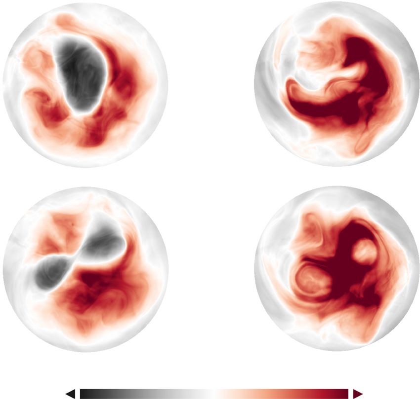
Reviews of Geophysics 10.1029/2020RG000708

Figure 7. Illustration of the evolution of the polar vortex during an SSW in the winter 2018/19. Panels show PV on the 850-K isentropic surface on six dates,
showing a sequence illustrating a displacement of the vortex off the pole with concomitant stripping away of vortex filaments into the surf zone. Once the
vortex is fully displaced off the pole (bottom middle). it then further splits into two smaller vortices (bottom right). From Baldwin et al. (2019) ©American
Meteorological Society. Used with permission.

 zonal wind anomalies is mechanistically similar to the QBO (Plumb & Semeniuk, 2003) but acts on a much
 faster time scale, on the order of days, not years.

 4.2. Bottom Up or Top Down: An Evolving Understanding on the Mechanism(s) Driving SSWs
 A “bottom up” perspective, focused on the role of enhanced tropospheric wave forcing, is inherent in
 Matsuno's seminal work on showing that SSWs are dynamically forced. Matsuno (1971) prescribed a
 switch-on planetary wave 2 forcing at the lower boundary (approximately the tropopause) of a GCM. The
 model produced a strong split SSW in response to this pulse from below.
 Matsuno's work suggests two key criteria for forcing an SSW. (1) SSWs only happen with sufficiently strong
 planetary wave forcing from the troposphere, and (2) SSWs require a pulse of anomalously strong wave
 forcing from the troposphere to initiate. Support for the first criterion includes the simple observation that
 warming events are much more prevalent in the NH versus SH. Additional support for a necessary minimum
 amount of wave forcing from the troposphere was established in a conceptual model developed by Holton
 and Mass (1976), who sought to distill an SSW down to its most basic elements.
 The Holton and Mass model consists of a single planetary wave of constant amplitude, prescribed as
 input forcing to the stratosphere at its lower boundary. The mean flow (i.e., the vortex) exists either in a
 strong state with weak wave amplitudes (corresponding to weak wave-mean flow interaction), or a weak
 state with strong wave amplitudes (corresponding to strong wave-mean flow interaction similar to the
 dynamics involved in SSWs). More recently, idealized GCM studies have found a sharp increase in SSW
 frequency as planetary-scale zonal asymmetries in the underlying flow are increased, either by topography

BALDWIN ET AL. 12 of 37

Reviews of Geophysics 10.1029/2020RG000708

 (e.g., Gerber & Polvani, 2009; Taguchi & Yoden, 2002) or thermal perturbations (Lindgren et al., 2018),
 though both topography and land-sea contrast may need to be present if represented in a realistic manner
 (Garfinkel et al., 2020).
 The second criterion in the Matsuno model—that SSWs are driven by an exceptional pulse of wave activity
 from the troposphere—is supported by the fact that SSWs are often preceded by blocking events, which
 amplify the tropospheric wave activity (e.g., Martius et al., 2009; Quiroz, 1986). This has led researchers to
 look for tropospheric precursor events that potentially give rise to additional planetary wave fluxes entering
 the stratosphere (e.g., Cohen & Jones, 2011; Garfinkel et al., 2010; Sun et al., 2012).
 Palmer (1981) suggested that the stratospheric vortex may need to be “preconditioned” to accept a pulse of
 wave activity, based on observations of the 1979 event, a topic further explored by McIntyre (1982). Various
 studies have suggested that the strength and size of the vortex play a critical role in allowing wave activity
 to penetrate deep into the stratosphere (Albers & Birner, 2014; Jucker & Reichler, 2018; Kuttippurath &
 Nikulin, 2012; Limpasuvan et al., 2004; Nishii et al., 2009).
 Newman et al. (2001) and Polvani and Waugh (2004) pointed out that a single precursor event will likely
 not cause sufficient deceleration of the stratospheric polar vortex; rather, it is the accumulated wave forcing
 over 40–60 days that needs to be anomalously strong to cause enough deceleration to reverse the zonal mean
 flow around the polar cap. Sjoberg and Birner (2012) further pointed out that sustained forcing that lasts for
 at least 10 days, but does not need to be anomalously strong, is crucial for forcing SSWs. Processes that can
 lead to such a sustained increase in wave forcing from the troposphere are discussed in section 5.
 Preconditioning suggests that the state of the stratospheric vortex impacts its receptivity to accept waves
 from the troposphere. The “top down” perspective takes this view to the extreme, supposing that fluctuations
 in tropospheric wave forcing do not play an important role at all. Rather, as long as the background wave
 fluxes entering the stratosphere are strong enough (such as provided by the climatological conditions in NH
 winter), the stratosphere is capable of generating SSWs on its own.
 The top down perspective has often been framed in the context of resonant growth of wave disturbances
 (e.g., Clark, 1974; Tung & Lindzen, 1979b). In a particularly insightful incarnation of this mechanism,
 the wave-mean flow interaction causes the vortex to tune itself toward its resonant excitation point
 (Matthewman & Esler, 2011; Plumb, 1981; Scott, 2016). Support for this perspective comes from idealized
 numerical model experiments that show that the stratosphere is capable of controlling the upward wave
 activity flux near the tropopause (Hitchcock & Haynes, 2016; Scott & Polvani, 2004, 2006) and that strato-
 spheric perturbations can trigger SSWs even when the tropospheric wave activity is held fixed (de la Cámara
 et al., 2017; Sjoberg & Birner, 2014).
 Preconditioning of the polar vortex, i.e., wave driving that brings it to the critical state, would clearly play
 a key role in this mechanism, suggesting that SSWs could potentially be predicted in advance, even in the
 limit where they are entirely controlled by the state of the stratospheric vortex.
 The bottom up and top down SSW mechanisms are associated with a different expected lag-lead relation-
 ship in upward wave energy propagation (i.e., the Eliassen-Palm flux) between the tropospheric source and
 stratospheric sink. Events forced by tropospheric waves will be preceded by a build up of wave activity over
 time, while self-tuned resonant SSWs would be characterized by nearly instantaneous wave amplification
 throughout an extended deep layer, and no lag between troposphere/tropopause and stratosphere.
 In this context, it is important to note that fluctuations in the upward wave flux at 100 hPa are not generally
 representative of fluctuations in the troposphere below (de la Cámara et al., 2017; Jucker, 2016; Polvani &
 Waugh, 2004). The typical tropopause pressure over the extratropical atmosphere during winter is around
 300 hPa, as shown in Figures 2 and 3. That is, wave flux events at 100 hPa can generally not be interpreted as
 tropospheric precursor signals because two thirds of stratospheric mass is below the height of the 100-hPa
 surface. Nevertheless, enhancements of upward wave fluxes from the troposphere at sufficiently long time
 scales (e.g., associated with climate variability extending over winter) tend to cause enhanced wave flux
 across 100 hPa into the polar vortex, which increases the likelihood for SSWs (as discussed in section 5).
 Evidence supporting both the bottom up and top down pathways has been observed, but it has become clear
 that the second criterion suggested by the Matsuno (1971) model—that the troposphere must drive an SSW
 with a pulse of enhanced wave activity—is not necessary. Birner and Albers (2017) found that only one third

BALDWIN ET AL. 13 of 37

Reviews of Geophysics 10.1029/2020RG000708

 Table 1
 Revisiting the QBO-SSW Relationship During 1958–2019, Based on the Dates
 Computed by Charlton and Polvani (2007) for 1958–2001 and by Rao
 et al. (2019) for 2002–2018 With NCEP/NCAR Reanalysis Data
 QBO-SSW relationship
 QBO phase Winter no. SSW no. SSW frequency
 EQBO (QBO50 ≥ 5) 20 18 0.9*
 WQBO (QBO50 ≤ -5) 36 18 0.5
 Neutral (|QBO50| < 5) 6 1 0.17*
 Total 62 37 0.60
 Note. The first column is the QBO phase. The second column is the corre-
 sponding composite size total winter (November–February mean) size. The
 third column is the number of SSWs events for that composite size, and the
 fourth column is the SSW frequency (units: events times per year). The unit
 of QBO50 is ms−1 . Significance for this and following tables is computed
 based on the following Monte Carlo test: SSWs are randomly assigned to win-
 ters while maintaining the overall SSW frequency, and then the frequency of
 SSWs for each phase is computed. This procedure is repeated 10,000 times, to
 which the observed SSW frequency is compared. If the observed frequency is
 less than 2.5%(5%) of the random samples, or greater than 97.5%(95%), then
 we can reject a null hypothesis of no relationship at the 95% or 90% confi-
 dence levels, which are indicated on the table with bold and a star. Reprinted
 with permission from Rao et al. (2019). EQBO = easterly phase of QBO;
 WQBO = westerly phase of QBO.

 of SSWs can be traced back to a pulse of extreme tropospheric wave fluxes. Roughly two thirds of observed
 SSWs are more consistent with the top-down category or do not fit into either prototype (i.e., tropospheric
 wave fluxes are anomalously strong but not extreme). Similar ratios have been observed in modeling studies
 by White et al. (2019) and de la Cámara et al. (2019), although results from mechanistic GCM experiments
 by Dunn-Sigouin and Shaw (2020) reemphasize the role of tropospheric wave fluxes.
 It also appears that the mechanism may vary with the type of warming. While Matsuno (1971) prescribed
 a wave 2 disturbance, it appears that wave 1 (displacement) events tend to be associated with the slow
 build up of wave activity, better matching the bottom-up paradigm, although resonant behavior has also
 been suggested for displacement events (Esler & Matthewman, 2011). Split, or wave 2, events are more
 instantaneous in nature (Albers & Birner, 2014; Watt-Meyer & Kushner, 2015), more closely matching the
 top-down paradigm.

 5. External Influences on SSWs
 Because there have only been around 40 observed SSWs between 1958 and 2019, it is challenging to quantify
 and/or establish statistically robust changes in frequency of SSWs from external influences, especially if the
 observations show a subtle effect. Despite this difficulty, a range of external influences have been connected
 to SSWs, including the QBO, ENSO, the 11-year solar cycle, the MJO, and snow cover. Confidence in the
 robustness of such relationships is increased if there is a well described physical mechanism that is expected
 to produce the observed effect, for example, through changes in the propagation and breaking of Rossby
 waves in the stratosphere or the generation of planetary Rossby waves in the troposphere. Similarly, confir-
 mation of observed relationships in modeling studies also increases confidence that they are robust. Even
 more challenging is establishing relationships in the observations whereby two or more external influences
 act in concert (Salminen et al., 2020), a topic we return to in section 10.
 It has been recognized for 40 years that the stratospheric polar vortex is weaker during the easterly QBO
 winter than during the westerly QBO winter, known as the Holton-Tan relationship (Anstey & Shepherd,
 2014; Holton & Tan, 1980). The frequency of occurrence of SSWs during each QBO phase is shown in Table 1
 based on NCEP-NCAR reanalysis. SSW likelihood is higher during easterly QBO winters than during west-
 erly QBO phase (0.9 vs. 0.5 year), consistent with early studies (Labitzke, 1982; Naito et al., 2003). Models
 also simulate a weakened vortex and more SSWs during easterly QBO as compared to westerly QBO, though
 the magnitude of the effect tends to be somewhat weaker than that observed (e.g., Anstey & Shepherd, 2014;

BALDWIN ET AL. 14 of 37