Surround Inhibition Mechanism by Deep Learning
←
→
Page content transcription
If your browser does not render page correctly, please read the page content below
OUJ-FTC-3
                                            OCHA-PP-356

                                                  Surround Inhibition Mechanism by Deep Learning∗

                                            Naoaki Fujimoto1 , Muneharu Onoue2 , Akio Sugamoto3,4 , Mamoru Sugamoto5,† ,
                                                                                       and Tsukasa Yumibayashi6
                                                 1
                                                     Department of Information Design, Faculty of Art and Design, Tama Art University,
arXiv:1908.09314v1 [q-bio.NC] 25 Aug 2019

                                                                                   Hachioji, 192-0394 Japan
                                                          2
                                                            Geelive, Inc., 3-16-30 Ebisu-nishi, Naniwa-ku, Osaka, 556-0003, Japan
                                                               3
                                                                   Tokyo Bunkyo Study Center, The Open University of Japan (OUJ),
                                                                                      Tokyo 112-0012, Japan
                                                           4
                                                            Ochanomizu University, 2-1-1 Ohtsuka, Bunkyo-ku, Tokyo 112-8610, Japan
                                                     5
                                                         Research and Development Division, Apprhythm Co., Honmachi, Chuo-ku, Osaka,
                                                                                   541-0053 Japan
                                             6
                                                 Department of Social Information Studies, Otsuma Women’s University, 12 Sanban-cho,
                                                                                    Chiyoda-ku, Tokyo 102-8357, Japan

                                                                                                   Abstract
                                                                       In the sensation of tones, visions and other stimuli, the “surround in-
                                                                   hibition mechanism” (or “lateral inhibition mechanism”) is crucial. The
                                                                   mechanism enhances the signals of the strongest tone, color and other
                                                                   stimuli, by reducing and inhibiting the surrounding signals, since the
                                                                   latter signals are less important. This surround inhibition mechanism
                                                                   is well studied in the physiology of sensor systems.
                                                                       The neural network with two hidden layers in addition to input
                                                                   and output layers is constructed; having 60 neurons (units) in each of
                                                                   the four layers. The label (correct answer) is prepared from an input
                                                                   signal by applying seven times operations of the “Hartline mechanism”,
                                                                   that is, by sending inhibitory signals from the neighboring neurons and
                                                                   amplifying all the signals afterwards. The implication obtained by the
                                                                   deep learning of this neural network is compared with the standard
                                                                   physiological understanding of the surround inhibition mechanism.

                                                 ∗
                                                 On the basis of this paper, Mamoru Sugamoto gave a talk at the 33rd Annual Conference of the Japanese
                                            Society for Artificial Intelligence (JSAI 2019), held at Niigata, Japan on June 5, 2019
                                               †
                                                 mamoru.sugamoto@gmail.com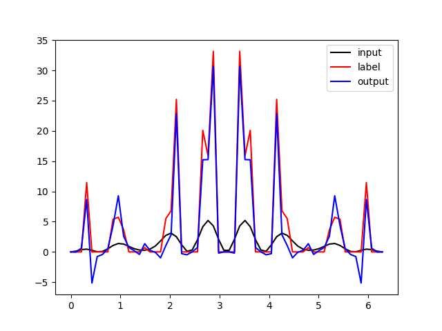
1     Introduction
The inhibitory influence between different sensory receptors is found in the eye of Limulus
(the horseshoe crab). Limulus has a pair of compound eyes. Each compound eye consists of
1000 ommatidia each of which is connected to a single nerve. Therefore, Limulus is the best
creature to study the interactions between different light censors.
   Hartline and his collaborators [1], [2] found by experiment that different ommatidia (light
sensors) are interacted, giving mutual inhibition, that is, the excitation signal eA of a sensor
A is inhibited from the neighboring sensor B, following the following linear equation:
                                                0             0
                         rA = eA − KAB × (rB − rB  ) θ(rB − rB  ),                            (1)
                          rB = eB − KBA × (rA − rA0 ) θ(rA − rA0 ).                           (2)

Here, eA,B is the excitation at A and B, induced when only A or B is stimulated. The rA,B
                                                                                             0
is the response of the sensory nerve, when they are stimulated at the same time. The rA,B
gives thresholds, by a step function θ(r − r 0 ) (= 1 if r − r 0 > 0, but else 0). The strength
of signal from a sensory nerve, is identified to the number of discharge of nerve impulses per
unit time.
    The inhibition (kinetic) coefficient KAB gives the rate of inhibition to the sensor A from
B. If A and B are the equal type, the reciprocal law KAB = KBA holds. Its value depends
on the pair of sensors, but is roughly 0.1 − 0.3 by experiment. In the later analysis, we use
0.25 for this inhibition coefficient.
    Suppose that the sensors, labeled by i, are lined laterally, while the layer is labeled by ℓ
to which the sensors are concentrated. Then, Eq. (1) becomes

                                                  ˙ − r 0 )j (ℓ) θ(rj − r 0 )(ℓ),
                                 X
                    ri (ℓ + 1) =     ri (ℓ) − Kij (r                     j                   (3)
                                 j

where we consider the response rj (ℓ) be the input signal to a receptor j located at layer ℓ,
and ri (ℓ + 1) is the output signal transferred to the receptor i located at the next layer ℓ + 1.
The 0-th layer can be the input layer, receiving the outside stimulus, ri (0) = ei .
    The same inhibition mechanism works for hearing. In this case, signals are transferred
from the cochlea where the voice sensor are placed, to cochlear nuclei, super olivary complex,
inferior colliculus, lateral geniculate body (LGB), before arriving at the auditory cortex. This
means there exist at least four layers between the input and output, in which neurons are
concentrated.
    If we use the “rectified linear unit (ReLU)” function defined by y = f (x) = ReLU(x) =
x × θ(x − x0 ), then we have
                                              X
                                                Kij × f (x − x0 )j (ℓ) .

                        xi (ℓ + 1) = xi (ℓ) −                                                  (4)
                                            j

This is identical to the neural network used by the deep learning (DL). In DL the adjustable
parameters are weights Wij , which is identical to the (kinetic) coefficients Kij of Hartline et
al., [1]. For the human hearing, the neural network having several layers are used.
    Now, we are ready to investigate by deep learning (DL) [3] how the sharpness of the
contrast in brightness, color, or sound tone can be achieved.

                                                2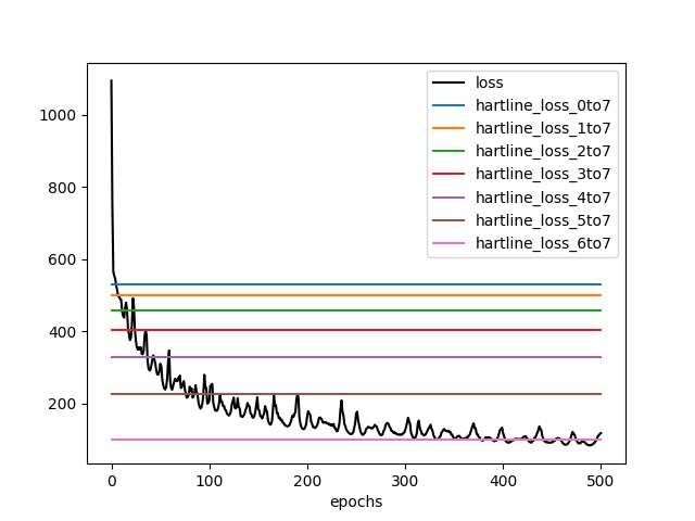
2     Implication by Deep Learning (DL)
We implement a neural network having two hidden layers, and the number of neurons (units)
in four layers of input, hidden1, hidden2 and output is all 60. The 1000 training data and
the 100 test data are prepared by random separation from 2000 data. Each datum and its
label (a correct answer to be attained from a datum by DL) are prepared by the Harline’s
observation. Given a one dimensional data of a certain signal (brightness or color of light,
frequency of sound, or else), as a sum of sin functions:
                                           5
                                                       !2
                                          X
                                X(x) =        an sin nx ,                                (5)
                                            n=1

where coefficients 0 ≤ {a1 , · · · , a5 } ≤ 1 are randomly generated, and x is the discretized
position of neurons, having 60 points {xi = 2πi    60
                                                      |i = 0, · · · , 59}. The “Hartline operation”
  ′
X = ĤX is defined by

                         X ′ (i) = λ · ReLU{Xi − κ(Xi+1 + Xi−1 )}.                             (6)

The label Y for a datum X is given by Y = (Ĥ)7 X with κ(= Hartline′ s K) = 0.25, and
λ = 2.
    The running of DL for 100,000 epochs, using sigmoid as the activation function and
the full Stochastic Gradient Descent method, yields the following
                                                              PN −1 epoch
                                                                    P59 dependence    of the
                                                            1                       2
loss function defined as the squared error, L(Xout , Y ) = 2N n=0 i=0 (Xout − Y ) , where
N = 100 is the total number of test data.
    See (Figure 1) which shows the decrease of loss function by epochs, as well as the inter-
mediate epochs of DL training, corresponding to the Hartline mechanism.

Figure 1: (Left): Loss as a function of epoch < 100,000; (Right): Horizontal lines show the
                       (n)
n-th Hartline loss L(XH , Y ) + 16.65 for epochs < 500.

   The left figure in (Figure 1) shows that the loss function decreases rapidly in the first
100 epochs, and it takes finally 16.65 at epoch 100,000 as the averaged value over the last
1000 epochs.
   It is important to compare the “Hartline’s mechanism” of the surround inhibition in
physiology [1], [2], with the implication obtained by DL of the neural network. We choose

                                                  3
six intermediate outputs, {X (1) , X (2) , · · · , X (6) } during the training of DL. The input datum
is X (0) and the output datum is Xout = X (7) . As for the Hartline mechanism, it gives the
(1) (2) (6) (n) (7)
six intermediate outputs by {XH , XH , · · · , XH }, where XH = (Ĥ)n X (0) , and XH = Y
is the label. Therefore, it is reasonable to select six intermediate epochs of the DL training
(n)
so that L(X (n) , Y ) = L(XH , Y ) + L(Xout , Y ) holds for n = 1, 2, · · · , 6, where the last term
in the r.h.s fills a gap 16.65 existing between the loss functions of Hartline and DL, even at
100,000 epochs’ running. From the the training data, we select the 6 intermediate epochs.
See the right figure in (Figure 1).
(n)
The loss functions between X (n) and XH , (n = 1, 2, · · · , 6) is a measure to understand
the difference between two mechanisms, Hartline’s physiological one and DL’s one. The data
(n)
shows intermediate epochs of DL which corresponds to the Hartline’s XH are 7, 11, 18, 37,
332, for n = 1, 2, 3, 4, 5, 6, respectively.
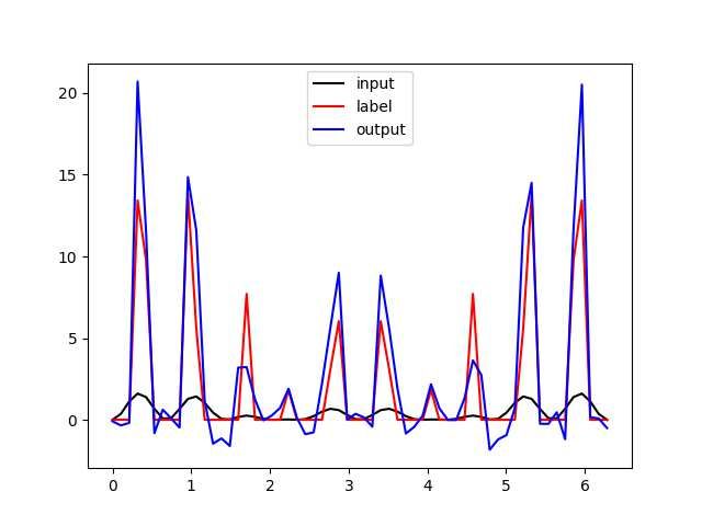
The performance can be seen visually from the following two samples among 100 test
data at 100,000 epoch, where the input, the label and the output signals are depicted by
black, red and blue colors, respectively. See (Figure 2). From the samples, we can see DL
Figure 2: Input (black), label (red) and output (blue) signals of two sample data among 100
test data at 100,000 epoch.
acquires an ability of making the sharp contrast to the input datum, resulting the output
datum in which the bumps are enhanced and strengthened.
3 Conclusion
The surround inhibition mechanism of sensory nerve system is studied by deep learning of
a neural network. The deep learning mechanism by this neural network is not necessary
equal to the standard one in physiology. More detailed comparison between DL and the real
sensory system is necessary, using the real data of the creature.
Acknowledgements
We are grateful to the members of the OUJ Tokyo Bunkyo Field Theory Collaboration for
fruitful discussions.
4References
[1] (Vision): H. K. Hartline, H. G. Wagner, and F. Ratliff, J. Gen. Physiol. 39 (1956) 651;
H. K. Hartline and F. Ratliff, i.b.d. (1957) 357; i.b.d. 41 (1958) 1049; D. H. Hubel and
T. N. Wiesel, J. Physiol. 148 (1959) 574;
(Audition): E. G. Wever, M. Lawrence, and G. von Békésy, Proc. N. A. S. 40 (1954)
508, H. Helmholtz, “On the Sensations of Tones” Dover Pub. (1885); G. von Békésy
and E. G. Wever, “Experiments in Hearing”, New York MacGraw-Hill Pub. (1960).
[2] M. Takagi, “Sensonary Physiology-Illustrated”, Shokabo Publishing (1989); A. Ogata,
“Musical Temperamant and Scale” revised version (2018).
[3] Y. LeCun, Y. Bengino and G. Hinton, Nature 521 436 (2015); K. Saitoh, ‘Deep
Learning-theory and implementation by Python-’, O’Reilly Japan (2016); Y. Sugu-
mori, “Deep Learning-time series date processing by TensorFlow and Keras-”, Mynavi
Publisher (2017).
5You can also read