Synthetic Aperture Radar (SAR) & Google Earth Engine - NASA

Page created by Carol Juarez

Science

English

Like
Share
Embed
Fullscreen
Slides
Download HTML
Download PDF
Abuse

←

→

Page content transcription

If your browser does not render page correctly, please read the page content below

Synthetic Aperture Radar (SAR) & Google Earth Engine - NASA

https://ntrs.nasa.gov/search.jsp?R=20200001565 2020-06-26T21:51:26+00:00Z

 Workshop:
 Synthetic Aperture Radar (SAR) &
 Google Earth Engine
 Source: ESA

Andrea Puzzi Nicolau
Amazonia Regional Science Associate
NASA SERVIR Science Coordination Oﬃce
Earth System Science Center
University of Alabama in Huntsville

Synthetic Aperture Radar (SAR)

Synthetic Aperture Radar (SAR)

Begin here

Radar → What’s the acronym?

Radar → What’s the acronym?

RAdio Detection And Ranging

Radar → What’s the acronym?

RAdio Detection And Ranging

What does SAR see?

● Structure
● Moisture

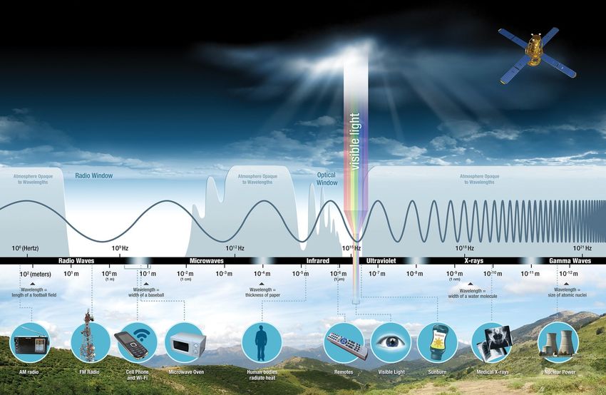
Electromagnetic Spectrum

Source: National Aeronautics and Space Administration, Science Mission Directorate. (2010).
Introduction to the Electromagnetic Spectrum. Retrieved [insert date - e.g. August 10, 2016],
from NASA Science website: http://science.nasa.gov/ems/01_intro

Radar Microwave Spectrum (approximately)
Band Frequency Wavelength General Application
 Ka 27 – 40 GHz 1.1 – 0.8 cm Rarely used for SAR (airports surveillance)

 K 18 – 27 GHz 1.7 – 1.1 cm Rarely used for SAR (H2O absorption)

 Ku 12 – 18 GHz 2.4 – 1.7 cm Rarely used for SAR (satellite altimetry)

 X 8 – 12 GHz 3.8 – 2.4 cm High-resolution SAR (urban monitoring; ice and snow; little penetration into
 vegetation cover; fast coherence decay in vegetated areas)

 C 4–8 GHz 7.5 – 3.8 cm SAR workhorse (global mapping; change detection; monitoring of areas with
 low to moderate vegetation; improved penetration; higher coherence); Ice,
 ocean, maritime navigation
 S 2–4 GHz 15 – 7.5 cm Little but increasing use for SAR-based Earth observation; agriculture
 monitoring (NISAR will carry an S-band channel; expands C-band
 applications to higher vegetation density)
 L 1–2 GHz 30 – 15 cm Medium resolution SAR (geophysical monitoring; biomass and vegetation
 mapping; high penetration; InSAR)
 P 0.3 – 1 GHz 100 – 30 cm Biomass. First P-band spaceborne SAR will be launched ~2020; vegetation
 mapping and assessment. Experimental SAR

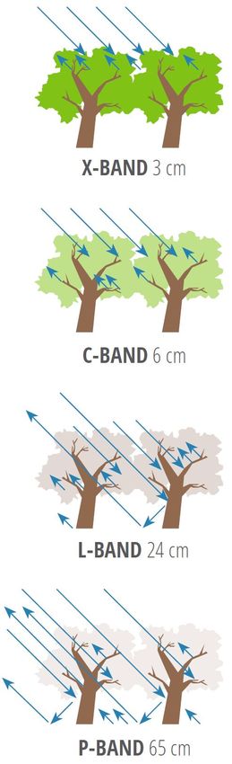
Radar Microwave Spectrum (approximately)
Band Frequency Wavelength General Application
 Ka 27 – 40 GHz 1.1 – 0.8 cm Rarely used for SAR (airports surveillance)

 K 18 – 27 GHz 1.7 – 1.1 cm Rarely used for SAR (H2O absorption)

 Ku 12 – 18 GHz 2.4 – 1.7 cm Rarely used for SAR (satellite altimetry)

 X 8 – 12 GHz 3.8 – 2.4 cm High-resolution SAR (urban monitoring; ice and snow; little penetration into
 vegetation cover; fast coherence decay in vegetated areas)

 C 4–8 GHz 7.5 – 3.8 cm SAR workhorse (global mapping; change detection; monitoring of areas with
 low to moderate vegetation; improved penetration; higher coherence); Ice,
 ocean, maritime navigation
 S 2–4 GHz 15 – 7.5 cm Little but increasing use for SAR-based Earth observation; agriculture
 monitoring (NISAR will carry an S-band channel; expands C-band
 applications to higher vegetation density)
 L 1–2 GHz 30 – 15 cm Medium resolution SAR (geophysical monitoring; biomass and vegetation
 mapping; high penetration; InSAR)
 P 0.3 – 1 GHz 100 – 30 cm Biomass. First P-band spaceborne SAR will be launched ~2020; vegetation
 mapping and assessment. Experimental SAR

SAR backscatter values are determined by the sensor and object characteristics

• Sensor characteristics:
 – Frequency/wavelength
 For time series analysis:
 – Polarization,
 Always use data with same characteristics
 – Incidence angle, To avoid errors in change detection
 – Slant-range direction

• Object characteristics:
 – Increase in soil and vegetation moisture increase in backscatter
 – Water bodies low response (dark image) - However, wind and ocean currents can increase backscatter
 response especially for short wavelengths (X, C bands)
 – For longer wavelengths, double-bounce effect under the canopy can increase the backscatter response

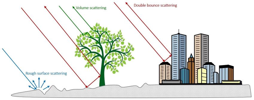
Scattering mechanisms
• Three main scattering mechanisms:
 Rough surface scattering: water, bare soils, paved surfaces - scattering strongly dependent on surface roughness
 and sensor wavelength
 Double bounce scattering: buildings, tree trunks, light poles, and other vertical structures - little wavelength
 dependence
 Volume scattering: Vegetation; dry soils with high penetration – strongly dependent on sensor wavelength and
 dielectric properties of medium

Polarizations

 HH HV

 Horizontal Transmit Horizontal Transmit
 Horizontal Receive Vertical Receive

 VV VH

 Vertical Transmit Vertical Transmit
 Vertical Receive Horizontal Receive

SAR polarimetry

• Single polarization (single pol):
 – VV or HH (or possibly HV or VH)

• Dual polarization (dual pol):
 – HH and HV, VV and VH, or HH and VV

• Quad polarization (quad pol, fully-polarimetric):
 – HH, VV, HV, and VH

The concept of Synthetic Aperture Radar

 Flight direction (along track)

 Antenna
 Footprint
 High resolution

 Combination of all acquisitions

Geometric distortions due to viewing geometry (side-looking)

 Foreshortening Layover Shadow
 • Sensor-facing slope • Mountain top overlain on • Area behind mountain
 foreshortened in image ground ahead of mountain cannot be seen by sensor
 • Foreshortening effects • Layover effects decrease • Shadow effects increase
 decrease with increasing with increasing look angle with increasing look angle
 look angle

Geometric terrain correction example
 Original Image

 Fuente: JAXA

Geometric terrain correction example
 Corrected Image

 Fuente: JAXA

Radiometric Terrain Correction
 ● Problem: Sensor facing slopes appear overly bright in radar images
 ● Cause: Pixel Size on sensor facing slopes is larger → more ground is integrated
 into pixel → brightness goes up

 Solution: Radiometric Terrain Correction (RTC)
 1. Using DEM and observation geometry, calculate exact equivalent area Aσ
 covered by each pixel
 2. Normalize radar cross section by Aσ to arrive at terrain normalized data

RTC example
 Image after GTC

 Fuente: JAXA

RTC example
 Image after RTC

 Fuente: JAXA

The inﬂuence of signal polarization

 Relative Scattering Strength by Polarization

● Rough Surface Scattering |SVV| > |SHH| > |SVH| or |SHV|

● Double bounce Scattering: |SHH| > |SVV| > |SVH| or |SHV|

● Volume Scattering: Main source of |SVH| and |SHV|

 Legend
 Low Radar Brightness (|S|) High Radar Brightness (|S|)

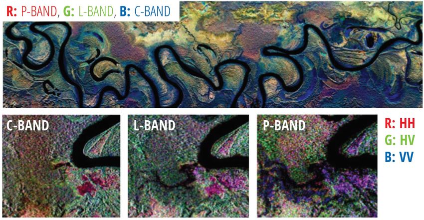
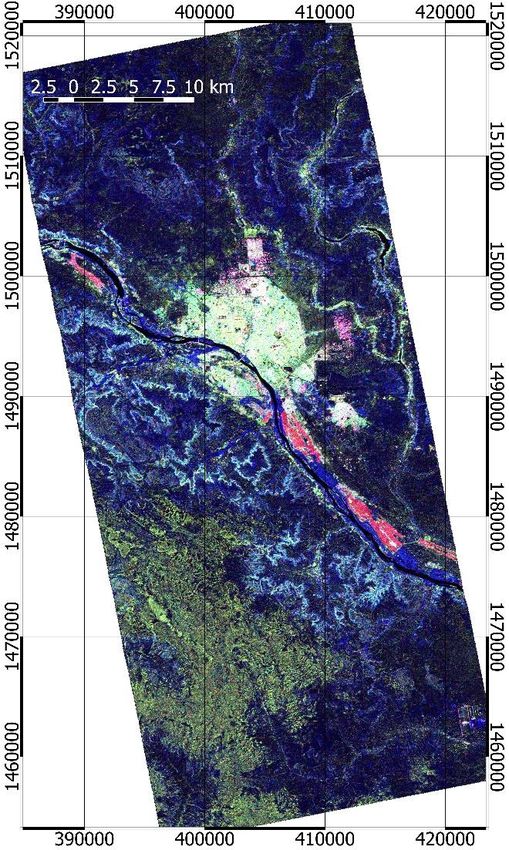
Polarimetric example for Niamey, Niger
 (a) (b) (c) (d)
 HH VV HV RGB

 Fully-polarimetric L-band SAR scenes from the ALOS PALSAR sensor over Niamey, Niger: from (a) to (c)
 scattering powers from |SHH|, |SVV| and |SHV|, respectively. (d) RGB color combination (|SHH|, |SHV|, |SVV|)

SAR backscatter response from Vegetation in different Wavelengths and
 Polarizations
Increase in penetration depth with an
 increase in wavelength

 Polarimetric responses and the medium characteristics are dependent on the sensor wavelength

Preprocessing steps, RTC and Geocoded Product
 WORKFLOW FOR RADIOMETRIC TERRAIN CORRECTION AND GEOCODING
 Read in
 SAR data

 Apply precise Load in
 orbit ﬁles DEM

 Radiometric Radiometric Terrain Geocoding/
 Multi-looking Speckle ﬁlter Geometric Terrain
 Calibration Correction (RTC) Correction
 Reduction in
 resolution to match Speckle noise
 DEM’s resolution reduction
 Linear to decibel
 OPTIONAL STEP
 conversion
 OPTIONAL STEPS

 Write data to
 GeoTIFF

Preprocessing steps, RTC and Geocoded Product
1. Apply precise orbit ﬁles: updates metadata with a more precise orbit
 information
2. Radiometric Calibration: Converts DN to backscatter (σo)
3. Multi-looking: Resolution reduction for DEM matching
4. Speckle Filter: Speckle noise reduction
5. Radiometric Terrain Correction (RTC): Backscatter intensity correction in pixels
 that were distorted by viewing geometry (radiometric terrain ﬂattening)
6. Geocoding/Geometric Terrain Correction (GTC): removes geometric image
 distortions due to viewing geometry

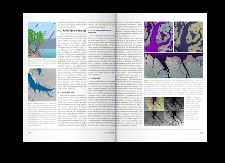
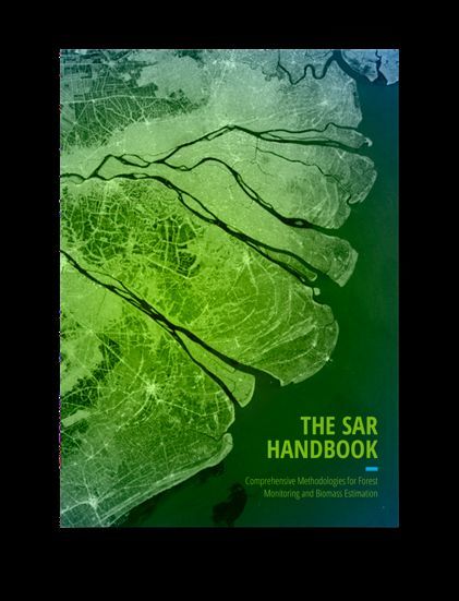
SAR Handbook: Comprehensive Methodologies for
Forest Monitoring and Biomass Estimation

 ▷ Freely-available eBook, interactive pdfs, and training modules;
 result of a 2-year joint collaboration between NASA SERVIR &
 SilvaCarbon
 ▷ Applied content, hands-on trainings to get started using SAR for
 forest monitoring, biomass estimation, mangrove extent, time
 series analysis
 ▷ Authored by world-renowned SAR experts from the NISAR Science
 Team, US Forest Service, academia
 ▷ Reviewed and tested by the SERVIR Global network
 ▷ Downloadable open-source scripts and sample datasets for a
 variety of forestry applications; useful for beginners to experts Selected pages from Ch. 6:
 Radar Remote Sensing of Mangrove
 Forests (by Dr. Marc Simard, Sr. Scientist &
 mangrove specialist, NASA Jet Propulsion
Download the SAR Handbook here: https://bit.ly/2UHZtaw Laboratory)
SAR Handbook training modules and more: https://bit.ly/2GeKvAN
For more information, visit the SERVIR website: SERVIRglobal.net
Contact: Africa Flores-Anderson (africa.ﬂores@nasa.gov)

Google Earth Engine

Google Earth Engine

● Planetary-scale cloud
 platform
● For access, processing, and
 analysis of multitemporal
 satellite data from different
 sources
● Entire collections such as
 the Landsat archive are
 already there
● JavaScript or Python API
● Shareable scripts
● Own data upload Source: Gorelick et al., 2017

Google Mission Statement

 "To organize the world's information and make it
 universally accessible and useful."

Source: Nick Clinton (https://goo.gl/n5Gh5Q)

The Earth Engine Data Catalog

Landsat & Sentinel 1, 2 MODIS Vector Data Terrain & Weather & Climate
 10-30m, weekly 250m daily WDPA, Tiger Land Cover NOAA NCEP, OMI, ...

 ... and upload your own vectors and rasters

 > 200 public datasets > 4000 new images every day
 > 5 million images > 7 petabytes of data

 Source: Nick Clinton (https://goo.gl/n5Gh5Q)

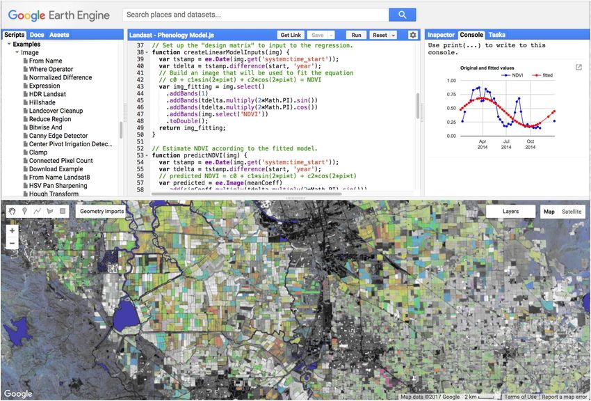
The Earth Engine Code Editor
 Your Data Search Your Code Data Inspector
 API Docs Output Console

 Your Scripts & Batch Tasks
Example Scripts

 Drawing Tools Map

Source: Nick Clinton (https://goo.gl/n5Gh5Q)
 code.earthengine.google.com

Sentinel-1 Data in GEE

Sentinel-1 Data in GEE

● Logarithm scale (dB)
 ○ 10 x log10(σo)
 ○ Backscatter coeﬃcient σo

● Choose only one path direction
 (ascending or descending)

● Radiometric Terrain
 Flattening/Correction not applied in
 GEE
 ○ Can produce geocoding and radiometric
 errors

Sentinel-1 in GEE examples

https://bit.ly/35XVI3k

Script 1
Script 2
Script 3

Survey

menti.com

161761

Thank You!

 Source: ASF

Andrea Puzzi Nicolau
Amazonia Regional Science Associate
NASA SERVIR Science Coordination Oﬃce
Earth System Science Center
University of Alabama in Huntsville
andrea.puzzinicolau@nasa.gov
andrea.nicolau@uah.edu
 @puzzinicolau

Taller:
 Radar de Apertura Sintética (SAR) y
 Google Earth Engine
 Fuente: ESA

Andrea Puzzi Nicolau
Investigadora Asociada
NASA SERVIR Science Coordination Oﬃce
Earth System Science Center
University of Alabama in Huntsville

Synthetic Aperture Radar (SAR)

 Radar de Apertura Sintética

Synthetic Aperture Radar (SAR)

 Radar de Apertura Sintética

Empezar con esto

Radar → ¿Qué signiﬁca?

Radar → ¿Qué signiﬁca?

RAdio Detection And Ranging

Radar → ¿Qué signiﬁca?

RAdio Detection And Ranging

Detección y uso de ondas de radio

Radar → ¿Qué signiﬁca?

RAdio Detection And Ranging

 Fuente: NOAA

Detección y uso de ondas de radio

¿Que ve SAR?

● Estructura
● Humedad

Espectro electromagnético

Source: National Aeronautics and Space Administration, Science Mission Directorate. (2010).
Introduction to the Electromagnetic Spectrum. Retrieved [insert date - e.g. August 10, 2016],
from NASA Science website: http://science.nasa.gov/ems/01_intro

El Espectro de Microondas (aproximadamente)
Banda Frecuencia Longitud Aplicación típica
 Ka 27 – 40 GHz 1.1 – 0.8 cm Raramente se usa para SAR (vigilancia en aeropuertos)

 K 18 – 27 GHz 1.7 – 1.1 cm Raramente se usa para SAR (absorción de H2O)

 Ku 12 – 18 GHz 2.4 – 1.7 cm Raramente se usa para SAR (altimetría satelital)

 X 8 – 12 GHz 3.8 – 2.4 cm Resolución alta de SAR (monitoreo urbano; hielo y nieve; poca penetración
 en la cobertura vegetal; decadencia de coherencia rápida en áreas con
 vegetación)
 C 4–8 GHz 7.5 – 3.8 cm Caballo de batalla de SAR (mapeo global; detección de cambio; monitoreo
 de áreas con cobertura de vegetación de baja a moderada; penetración
 mejorada; mayor coherencia)
 S 2–4 GHz 15 – 7.5 cm Poco pero creciente uso en Obs. Terrestres basadas en SAR monitoreo de
 agricultura (NISAR tendrá Banda-S; expande aplicaciones de la banda-C para
 áreas con mayor densidad de vegetación)
 L 1–2 GHz 30 – 15 cm Resolución media de SAR (Monitoreo geofísico; mapeo de biomasa y
 vegetación; alta penetración; InSAR)
 P 0.3 – 1 GHz 100 – 30 cm Estimación de biomasa. El primer SAR satelital se lanzará en ~2020; mapeo
 y evaluación de vegetación. SAR experimental.

El Espectro de Microondas (aproximadamente)
Banda Frecuencia Longitud Aplicación típica
 Ka 27 – 40 GHz 1.1 – 0.8 cm Raramente se usa para SAR (vigilancia en aeropuertos)

 K 18 – 27 GHz 1.7 – 1.1 cm Raramente se usa para SAR (absorción de H2O)

 Ku 12 – 18 GHz 2.4 – 1.7 cm Raramente se usa para SAR (altimetría satelital)

 X 8 – 12 GHz 3.8 – 2.4 cm Resolución alta de SAR (monitoreo urbano; hielo y nieve; poca penetración
 en la cobertura vegetal; decadencia de coherencia rápida en áreas con
 vegetación)
 C 4–8 GHz 7.5 – 3.8 cm Caballo de batalla de SAR (mapeo global; detección de cambio; monitoreo
 de áreas con cobertura de vegetación de baja a moderada; penetración
 mejorada; mayor coherencia)
 S 2–4 GHz 15 – 7.5 cm Poco pero creciente uso en Obs. Terrestres basadas en SAR monitoreo de
 agricultura (NISAR tendrá Banda-S; expande aplicaciones de la banda-C para
 áreas con mayor densidad de vegetación)
 L 1–2 GHz 30 – 15 cm Resolución media de SAR (Monitoreo geofísico; mapeo de biomasa y
 vegetación; alta penetración; InSAR)
 P 0.3 – 1 GHz 100 – 30 cm Estimación de biomasa. El primer SAR satelital se lanzará en ~2020; mapeo
 y evaluación de vegetación. SAR experimental.

Los valores de retrodispersión SAR están determinados por las características
del sensor y del objeto

• Características del Sensor:
 Especialmente para análisis de series de tiempo:
 – frecuencia/longitud de onda de SAR, Usar datos con las mismas características del
 – Polarización de la señal SAR transmitida y recibida, sensor
 – ángulo de incidencia radar-suelo, Para evitar interpretaciones erróneas de
 – Y dirección de mirada del sensor características del sensor como cambio

• Características del Objeto:
 – Humedad en suelos y vegetación; agua estancada abierta y agua estancada debajo del dosel
 – Aumento en la humedad de los suelos y vegetación incrementa la retrodispersión SAR
 – Agua estancada abierta típicamente muy oscura - Sin embargo, viento y corrientes pueden agitar el
 agua y aumentar el brillo especialmente para observaciones de longitud de onda corta (banda X y C)
 – En longitudes de onda más largas, el efecto de doble rebote debajo del dosel puede tener una fuerte
 señal de retrodispersión

¿Cómo reacciona la señal del SAR?
• En la longitud de onda del radar, la dispersión es muy física y puede describirse como una serie de rebotes en
 las interfaces de dispersión
• Tres mecanismos principales de dispersión dominan:
 – Dispersión en superﬁcies (rugosas): agua, suelos desnudos, caminos – la dispersión depende en gran medida de
 la rugosidad de la superﬁcie y la longitud de onda del sensor
 – Dispersión de doble-rebote: Ediﬁcios, troncos de árboles, postes de luz – poca dependencia de la longitud de onda
 – Dispersión volumétrica: Vegetación; suelos secos con alta penetración – depende fuertemente de la longitud de
 onda del sensor y las propiedades dieléctricas del medio

Polarizaciones

 HH HV

 Transmisión Horizontal Transmisión Horizontal
 Recepción Horizontal Recepción Vertical

 VV VH

 Transmisión Vertical Transmisión Vertical
 Recepción Vertical Recepción Horizontal

Conﬁguraciones del sistema SAR polarimétrico

• Polarización única (single pol):
 – VV o HH (o posiblemente HV o VH)

• Polarización doble (dual pol):
 – HH y HV, VV y VH, o HH y VV

• Polarización cuádruple (quad pol) (totalmente polarimétrico):
 – HH, VV, HV, y VH

Formación de una apertura sintética - Principio SAR

Distorsiones geométricas como consecuencia del ángulo oblicuo

 Escorzo/perspectiva Inversión por relieve Sombra
 (foreshortening) (Layover) • Área detrás de la montaña no
 • Pendiente orientada al sensor • Cima de la montaña puede ser vista por el sensor
 acortada en la imagen sobrepuesta a la base delante • Estos efectos aumentan al
 • Estos efectos disminuyen al de la montaña aumentar el ángulo de mirada
 aumentar el ángulo de mirada • Estos efectos disminuyen al
 aumentar el ángulo de mirada

Ejemplo de Corrección geométrica del terreno
 Imagen Original

 Fuente: JAXA

Ejemplo de Corrección geométrica del terreno
 Imagen Corregida geométricamente

 Fuente: JAXA

Corrección Radiométrica del Terreno
 ● Problema: Las pendientes orientadas al sensor aparecen demasiado brillantes
 en las imágenes de radar
 ● Causa: El tamaño del píxel en las pendientes orientadas al sensor es mayor →
 más área es integrada al pixel → el brillo aumenta

 Solución: Corrección Radiométrica del Terreno (RTC, por sus siglas en inglés)
 1. Usando el DEM y observación geométrica, se calcula la área equivalente exacta
 cubierta por cada pixel
 2. Normaliza la sección transversal por la área equivalente exacta para llegar a
 datos normalizados del terreno

Ejemplo de Corrección geométrica del terreno
 Imagen después de GTC

 Fuente: JAXA

Ejemplo de Corrección geométrica del terreno
 Imagen después de RTC

 Fuente: JAXA

Dependencia polarimétrica de los principios de dispersión

 Fuerza de dispersión relativa por polarización

● Dispersión de la superfície pura: |SVV| > |SHH| > |SVH| o
 |SHV|

● Dispersión de doble rebote: |SHH| > |SVV| > |SVH| o |SHV|

● Dispersión volumétrica: fuente principal de |SVH| y |SHV|

 Leyenda
 Bajo brillo de radar (|S|) Alto brillo de radar (|S|)

Ejemplo de dispersión polarimétrica para Niamey, Níger
 (a) (b) (c) (d)
 HH VV HV RGB

Escena SAR de banda L completamente polarimétrica del sensor ALOS PALSAR sobre Niamey, Níger: de (a) a (c)
 se muestra la fuerza de dispersión de |SHH|, |SVV| y |SHV|. (d) muestra la combinación RGB (|SHH|, |SHV|, |SVV|)

Firmas SAR de Vegetación en Diversas Frecuencias y Polarizaciones
Aumento de la profundidad de penetración
 con la longitud de onda.

 El cambio de ﬁrma polarimétrica y las características de la cubierta inferior están expuestas a medida que aumenta la longitud de onda

Preparación de los datos, Procesamiento RTC y Producto Geocodiﬁcado
 FLUJO DE TRABAJO DE CORRECCIÓN RADIOMÉTRICA DEL TERRENO Y GEOCODIFICACIÓN
 Leer datos
 SAR

 Aplicar archivos de Cargar
 órbita DEM

 Corrección Geocodiﬁcación /
 Calibración Corrección
 Multi-looking Filtro de Moteado radiometrica del Geométrica del
 radiometrica
 terreno (RTC) Terreno
 Reduce la resolución
 para que coincida con Reduce ruido
 DEM Conversión lineal a
 PASOS OPCIONALES PASO OPCIONAL
 decibeles

 Escribir
 datos a
 GeoTIFF

Preparación de los datos, Procesamiento RTC y Producto Geocodiﬁcado
1. Aplicar archivos de órbita: actualiza los metadatos con información de órbita
 más precisa
2. Calibración radiométrica: cambia los número digitales para números de
 retrodispersión (σo)
3. Multi-looking: reduce la resolución para que coincida con el DEM y para reducir
 ruido
4. Filtro de Moteado: Reduce ruido
5. Corrección radiométrica del terreno (RTC): corrección de la intensidad de
 retrodispersión en pixels que fueron distorsionados por la geometría de
 observación (aplanamiento)
6. Geocodiﬁcación/Corrección geométrica del terreno (GTC): corrección de la
 posición de los pixels que fueron distorsionados por la geometría de
 observación

Manual SAR: Metodologías integrales para el
monitoreo forestal y la estimación de biomasa
 ▷ eBook de libre acceso, pdfs interactivos, módulos de
 entrenamiento; resultado de una colaboración conjunta de 2+ años
 entre NASA SERVIR & SilvaCarbon
 ▷ Contenido aplicado, entrenamientos prácticos para comenzar a
 usar SAR para monitoreo forestal, estimación de biomasa,
 detección de mangle, análisis de series de tiempo
 ▷ Escrito por expertos en SAR de renombre mundial del equipo
 Cientíﬁco de NISAR, Servicio Forestal de US, academia
 ▷ Revisado y probado por la red global de SERVIR
 ▷ Scripts de código abierto descargables y conjuntos de datos de
 muestra para una variedad de aplicaciones forestales; útil de
 Páginas seleccionadas del Cap. 6:
 principiantes a expertos Radar Remote Sensing of Mangrove
 Forests (by Dr. Marc Simard, Sr. Scientist &
 mangrove specialist, NASA Jet Propulsion
Descarga el Manual SAR aquí: https://bit.ly/2UHZtaw Laboratory)
Módulos de entrenamiento del Manual SAR y más: https://bit.ly/2GeKvAN
Para mayor información, visitor el sitio website de SERVIR @ SERVIRglobal.net
Contacto: Africa Flores-Anderson (africa.ﬂores@nasa.gov)

Google Earth Engine

Google Earth Engine

● Una plataforma en línea de
 escala planetária
● Para acceso, procesamiento
 y análisis multitemporal de
 datos satelitales de diversas
 fuentes
● Archivos completos como
 del Landsat ya están allá
● API en JavaScript o Python
● Compartimiento de scripts
● Carga de datos propios
 Fuente: Gorelick et al., 2017

Google Mission Statement

 "To organize the world's information and make it
 universally accessible and useful."

Fuente: Nick Clinton (https://goo.gl/n5Gh5Q)

Catálogo de Datos de Earth Engine

Landsat & Sentinel 1, 2 MODIS Datos Vectoriales Terreno & Datos Climáticos
 10-30m, semanalmente 250m diariamente WDPA, Tiger Cobertura del Suelo NOAA NCEP, OMI, ...

 ... y cargas sus propios datos vectoriales y rasters

 > 200 datasets públicos > 4000 nuevas imágenes diariamente
 > 5 millones de imágenes > 7 petabytes de datos

 Fuente: Nick Clinton (https://goo.gl/n5Gh5Q)

Earth Engine Editor de Código
 Tu Datos Buscas Su código Inspector de Datos
 Documentación Console de
 del API Resultados

 Tu Script & Tareas
 Ejemplos de
 Scripts
 Herramientas Mapa
 de dibujo

Fuente: Nick Clinton (https://goo.gl/n5Gh5Q)
 code.earthengine.google.com

Datos Sentinel-1 en GEE

Datos Sentinel-1 en GEE

● Escala logarítmica en decibeles (dB)
 ○ 10 x log10(σo)
 ○ Coeﬁciente de retrodispersión σo
● Elegir solamente un tipo de
 geometría de observación
 (ascending o descending)
● Corrección/Aplanamiento
 radiométrico de terreno no es
 aplicado en GEE
 ○ Puede traer errores de geocodiﬁcación e de
 radiometría

Ejemplos para Sentinel-1 en GEE

http://bit.ly/SERVIRAmazoniaEE

Script 1
Script 2
Script 3

Retroalimentación

menti.com

161761

iGracias!

 Fuente: ASF

Andrea Puzzi Nicolau
Investigadora Asociada
NASA SERVIR Science Coordination Oﬃce
Earth System Science Center
University of Alabama in Huntsville
andrea.puzzinicolau@nasa.gov
andrea.nicolau@uah.edu
 @puzzinicolau

You can also read