THE CHANGE ON FLOODING - WORKSTREAM 4: RESEARCH REPORT IMPACT OF CLIMATE - CSIR

THE IMPACT OF CLIMATE
CHANGE ON FLOODING
WORKSTREAM 4: RESEARCH REPORT

2019

Authors David Le Maitre and Ilse Kotzee
 Date 2019
 ToDB reference CSIR/NRE/ECOS/ER/2019/0001/C
 Le Maitre, D & Kotzee, I. 2019. Green Book – The impact of climate
 Suggested citation
 change on flooding. Technical report, Pretoria: CSIR

Disclaimer and acknowledgement: This work was carried out with the aid of a grant from the CSIR Long-term
Thematic Programme, Pretoria, South Africa and the International Development Research Centre, Ottawa,
Canada. The views expressed herein do not necessarily represent those of the IDRC or its Board of Governors.

 2

TABLE OF CONTENTS tents
1 INTRODUCTION ............................................................................................. 6

2 BACKGROUND .............................................................................................. 7

 2.1 Flood hazard ......................................................................................................... 7

 2.1.1 Regionalising observed data .......................................................................... 7

 2.1.2 Design flood estimation .................................................................................. 8

 2.1.3 Assessing catchment responsiveness............................................................ 9

 2.1.4 Simulating floods.......................................................................................... 11

 2.1.5 Summary ..................................................................................................... 11

 2.2 Flood vulnerability ................................................................................................ 13

 2.2.1 Physical exposure ........................................................................................ 13

 2.2.2 Assets exposed ........................................................................................... 14

 2.2.3 Participatory approaches ............................................................................. 15

 2.2.4 Summary ..................................................................................................... 15

3 METHODOLOGY .......................................................................................... 16

 3.1 Current climate and hydrological characteristics .................................................. 16

 3.2 Future climates and flood hazard ......................................................................... 16

 3.3 Flood hazard ....................................................................................................... 17

 3.4 Flood exposure .................................................................................................... 21

4 RESULTS ...................................................................................................... 21

 3

4.1 Climate and hydrological characteristics .............................................................. 21

 4.2 Projected increases in extreme daily rainfall ........................................................ 25

 4.3 Flood Hazard Index ............................................................................................. 27

 4.4 Cederberg and Dihlabeng Local Municipalities .................................................... 30

5 CONCLUSION .............................................................................................. 39

6 REFERENCES .............................................................................................. 41

TABLE OF FIGURES
Figure 1: Diagram summarising the steps and inputs in the calculation of the flood hazard. 19
Figure 2: 50-year return period design on day (daily) rainfall for South Africa (Schulze et al.,
2008). The class intervals are based on a geometric scale to reduce the influence of extreme
values ................................................................................................................................. 22
Figure 3: The modelled highest daily stormflow in a 10 year period (Schulze et al., 2008). The
class intervals are based on a geometric scale to reduce the influence of extreme values. . 23
Figure 4: The variability in the stormflow between years (inter-annual) as a percentage of the
mean stormflow (i.e. the Coefficient of Variation as a percentage) (Schulze et al., 2008). ... 24
Figure 5: The regionalised K-ratio i.e. the ratio of the flood peak in m3/sec to the average
annual flow in m3/sec for catchments in South Africa, Lesotho and Swaziland (Kovács, 1988).
Digital version supplied by the Aurecon Group (Andre Görgens personal comm) ............... 25
Figure 6: The mean ratio of the near-future (2021-2050) and current (1971-2000) extreme
daily rainfall (95th percentiles) for each quinary catchment. Values greater than 1.0 indicate
an increase in the extreme daily rainfall. ............................................................................. 26
Figure 7: The mean ratio of the near-future (2070-2099) and current (1971-2000) extreme
daily rainfall (95th percentiles) for each quinary catchment. Values greater than 1.0 indicate
an increase in the extreme daily rainfall. ............................................................................. 27
Figure 8: The Flood Hazard Index calculated by the SCIMAP model for the primary catchment
area U showing the mean values per quinary catchment. Class intervals based on the
standard deviation of the mean values per quinary catchment. ........................................... 28
Figure 9: The mean flood hazard calculated by the SCIMAP model for the primary catchment
area X (Inkomati River System) for each quinary. Class intervals based on the standard
deviation of the mean values per quinary catchment. .......................................................... 29

 4

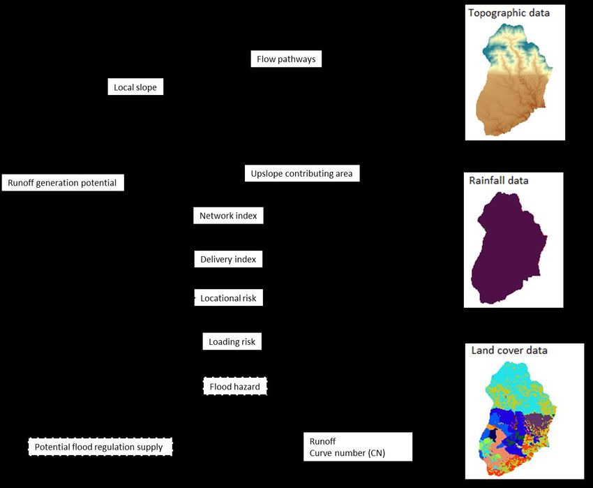
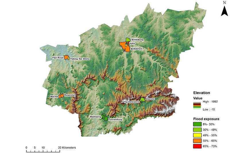
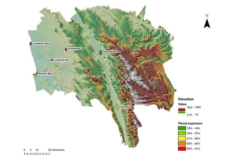
Figure 10: Mean Flood Hazard Index (FHI) per quinary (5th order) catchment based on the
SCIMAP model run at the secondary catchment level. Class intervals based on the standard
deviation of the mean FHI for the quinary catchments......................................................... 30
Figure 11: The Cederberg Municipality showing the settlements and the flood hazard modelled
for each one based on the SCIMAP model. ........................................................................ 31
Figure 12: The proportions of the different settlements that are exposed (i.e. situated within
10 m of the estimated river level). ....................................................................................... 32
Figure 13: The land cover in the areas situated less than 10 m above the level of the rivers
next to or passing through the settlements. Classes in the 2013/14 land cover (GTI, 2015)
were combined into the main ones form the risk perspective .............................................. 33
Figure 14: Cederberg Municipality showing the 1-day design rainfall (50 year return period)
for each of the quaternary catchments. Data from Schulze et al. (2008). ............................ 34
Figure 15: The Cederberg Municipality showing the mean FHI estimated by the SCIMAP
model for the quinary catchments in this area. .................................................................... 35
Figure 16: Dihlabeng Municipality showing the settlements and the flood hazard modelled for
each one based on the SCIMAP model............................................................................... 36
Figure 17: The proportions of the different settlements that are exposed (i.e. situated within
10 m of the estimated river level). ....................................................................................... 37
Figure 18: The land cover in the areas situated less than 10 m above the level of the rivers
next to or passing through the settlements. Classes in the 2013/14 land cover (GTI, 2015)
were combined into the main ones form the risk perspective. ............................................. 37
Figure 19: Dihlabeng Municipality showing the 1-day design rainfall (50 year return period) for
each of the quaternary catchments. Data from Schulze et al. (2008). ................................. 38
Figure 20: The Dihlabeng Municipality showing the mean FHI estimated by the SCIMAP model
for the quinary catchments in this area. Note that the class intervals differ a little from those in
the national level map ......................................................................................................... 39

LIST OF TABLES
Table 1: Hydrologic soil groups identified from soil textures ................................................ 20

 5

1 INTRODUCTION

Like many other countries, South Africa has a history of floods ranging from minor, local events
through to national disasters with widespread flooding generated by extreme events such as
cut-off lows and cyclones, the most recent one being cyclone Dineo in February 2017 (Davis-
Reddy and Vincent, 2017; Holloway et al., 2010; Kovács, 1988; Lund, 1984; Pharoah et al.,
2016; Pyle and Jacobs, 2016; Roberts and Alexander, 1982; Sakulski, 2007; van Niekerk et
al., 2016). Some information on the location of floods in southern Africa is available from the
 1
South African Weather Service , the Dartmouth Flood Observatory
(http://floodobservatory.colorado.edu/), datasets on global disaster hotspots (Dilley et al.,
2005), and the Aqueduct Global Flood Analyser (see
http://floods.wri.org/#/country/209/South%20Africa) (Ward et al., 2013; Winsemius et al.,
2015) and other databases.

Flood risk, like many other risks, can be disaggregated into two main components (Balica et
al., 2013):
  Flood hazard which focuses on the nature of the flood events and includes the
 likelihood and the severity of flood events

  Flood vulnerability which focuses on the effects of flood events on people, their
 livelihoods and infrastructure, and includes the degree of exposure, alternatively the
 magnitude of the consequences, and the resources available for them to recover
 from the flood.

1
 http://saweatherobserver.blogspot.co.za/search/label/flood%20damage

 6

2 BACKGROUND

2.1 Flood hazard

Along the coast flooding can be caused by high tides, storm surge and strong winds forming
high energy waves and, thus, increased wave run-up. Inland floods are caused by large
volumes of water which are generated by rainfall events. Both kinds of floods can occur
together when the same storm drives coastal flooding and inland flooding and the two combine
in estuarine environments. Inland floods are generated by rainfall in various ways including:
  very intense, short duration rainfall events which rapidly saturate (saturation excess)
 or exceed the ability of the soils to absorb the water (infiltration excess) (Beven,
 2004; Manfreda et al., 2010) and result in short duration flash floods; or

  longer, less intense rainfall events, or a sequence of events which also saturate
 catchments and can result in long duration floods; or

  groundwater table rises in response to rainfall recharge (Musungu et al., 2012).

The focus of this document is on floods generated by surface water (fluvial or river-related
floods) but the third cause is important in certain areas such as the Cape Flats near Cape
Town. The methods for doing flood hazard assessments can be broadly divided into two
categories – those based on analyses of observed or modelled floods and those based on
observed or statistically predicted rainfall events (Smithers, 2012; Smithers and Schulze,
2003).

2.1.1 Regionalising observed data

Approaches have been developed using observed flood data which are then turned into
regional estimates so they can be used in flood risk assessments (Benjamin, 2008; Smithers
and Schulze, 2003; van Bladeren et al., 2007). Key weaknesses are that: (a) they do not give
an estimate of the frequency of that flood (Van Bladeren et al., 2007); and (b) they are based
on data from a particular catchment with specific properties and have to be generalised for
regional use although this effect is reduced when data from sufficient catchments within a
region are available (Kovács, 1988).

 7

The regional maximum flood (RMF) approach used by Kovács (1988) applied an equation
developed from an international study which linked upstream catchment area and observed
maximum flood peaks (Francou and Rodier, 1969). The K-ratio derived from the equation
represents the ratio of the maximum flood to the normal runoff. The upstream areas are
divided into three ranges: areas 100-500 km2 where the flood
ratio is the catchment characteristics and the rainfall; and a “transition zone” between 1 and
100-500 km2 where there is mixed response (Kovács, 1988). In South Africa the transition
zone appeared to apply up to 200 km2 and the reliability of the estimated K-ratio decreased
as catchment area decreased. The K-ratios were generalised to regions using information on
the catchment characteristics and 3-day rainfall to create a map for the country (Kovács,
1988). There have been a number of local refinements of this approach, some combined with
models (Nortje, 2010; Pegram and Parak, 2004; Vischel et al., 2008), but only one has used
sites from across the whole country (Görgens, 2007). There have been similar approaches
which incorporated flood frequency but they have also only examined certain catchments
(Smithers et al., 2015; Van Bladeren et al., 2007). A couple of studies have derived
regionalised flood magnitude and frequency information for southern Africa but generally at a
relatively coarse resolution (Haile, 2011; Kachroo et al., 2000; Mkhandi et al., 2000), so the
Kovács (1988) estimates are still used.

2.1.2 Design flood estimation

One of the standard modelling approaches, design flood estimation, was developed primarily
for assisting engineers in designing structures to cope with predicted volumes of flood water
(Smithers, 2012; Smithers and Schulze, 2003). This generally uses a simplified representation
of the catchment and its potential to generate floods based on a variety of approaches. It is
used for detailed analyses of single events, typically in small catchments, and uses statistical
analyses of the regionalised characteristics of the rainfall which provide design rainfall
amounts as inputs (Knighton and Walter, 2016; Knoesen and Smithers, 2008; Smithers, 2012;
Smithers and Schulze, 2004, 2003; Van Bladeren et al., 2007). The most common modelling
approaches used for event based analysis in South Africa are the Rational, Unit Hydrograph
and SCS methods (Smithers, 2012). A disadvantage of these approaches is that they focus
mainly on the rainfall while largely ignoring catchment behaviour, a limitation which becomes
more important as catchment heterogeneity increases. Software packages are available to do
this type of modelling under local conditions (Gericke and Du Plessis, 2013; Smithers, 2012;
Smithers and Schulze, 2003).

 8

An alternative method of estimating the flood hazard involves generating time series of river
flows using a simulation model (Smithers et al., 2013):
  Selecting, setting-up and calibrating a suitable hydrological model for the catchment
 area in which the settlement is located. The model should be able to run on a daily
 time step (preferably hourly), should be able to represent the catchment properties
 and behaviour adequately and needs to be able to simulate the runoff following rainfall
 events. Once it is set up, the outputs are compared with observed data from the
 catchment and the parameters in the model are adjusted until its simulated flows
 match the observed flows sufficiently accurately (typically within 10%), a process
 known as calibration. The model can be run using design rainfall data (Knighton and
 Walter, 2016; Knoesen and Smithers, 2008; Smithers and Schulze, 2004, 2003) or a
 range of historical high rainfall events to generate time series of runoff volumes. The
 ACRU model was tested in the Thukela River catchment and was found to perform
 reasonably well at simulating flood volumes (Smithers et al., 2013)
  These runoff volumes can then be used as inputs to a hydraulic flow-routing model
 which uses detailed information on topography and roughness of the river floodplain
 and adjacent areas to predict the depth (extent) and duration of the flood for vulnerable
 areas of the catchment (Zerger and Wealands, 2004). This model should preferably
 be calibrated as well.

Some flood models can combine these two steps. Following such an approach in this study is
simply not feasible given the time required to source the necessary input datasets, calibrate
the models, run them and interpret the outputs. These kinds of issues are the main reason
why such an approach has not been applied across the country (Els and Van Niekerk, 2013).
The number and location of the settlements is not known at this stage and there are few
gauged catchments in the country, so it is likely that settlements will occur in catchments with
no observed flow records, and obtaining suitable rainfall datasets could be problematic.

2.1.3 Assessing catchment responsiveness

An alternative approach is needed which is able to use information on the characteristics of
the catchment to at least estimate its responsiveness to rainfall events whilst being applicable
to a range of catchments. It needs to be able to represent how rainfall event size, duration and
intensity interact with the characteristics of the catchment to influence its behaviour i.e. the
volume and rate of flow of the runoff. Key factors in catchment responsiveness are the

 9

topography, especially the steepness, the depth of the soils and the ability of the soils and
subsurface systems to take-up (capture) and store the rainwater (Beven, 1987; Görgens,
2007; Jencso and McGlynn, 2011; Kourgialas and Karatzas, 2011; McDonnell, 2009; Merz
and Blöschl, 2008a, 2008b; Sayama et al., 2011). Essentially this can be viewed as a
combination of the extent and sensitivity of the runoff generating areas (Cheng et al., 2014)
and the hydrological connectivity (the ease with which surface runoff moves across a
landscape) (Hahn et al., 2014; Kourgialas and Karatzas, 2011; Lane et al., 2009, 2003). The
RMF study took some catchment characteristics into account by including relief, catchment
orientation in relation to the movement of storm-generating weather systems, general soil
permeability, the main drainage network and any very large dams situated upstream (Kovács,
1988). The interpolation was based on mapped information on the different variables and
expert judgement. Other studies have used the catchment area (which is always significant),
mean annual precipitation, the river slope, mean annual rainfall and runoff, the longest stream
length, grouped veld (vegetation) types and grouped K-regions (Görgens, 2007; HRU, 1972;
Van Bladeren et al., 2007). One study found that including a range of catchment
characteristics did not improve the performance of a regional flood frequency analysis
(Smithers et al., 2015). The importance of considering the hazard is taken into account by the
Flood Vulnerability Index which uses physical and environmental indicators for different sizes
of study areas (river basin to urban area), including rainfall characteristics, land cover,
topography, river flow characteristics and dam storage upstream (Balica and Wright, 2010).

Catchment responsiveness also varies depending on its initial state prior to a given rainfall
event, particularly how “wet” it was prior to the rainfall event of interest (antecedent wetness)
(Brocca et al., 2011; Longobardi et al., 2003). Typically, the wetter it is the more likely it is to
produce a greater volume of runoff. The more responsive a catchment is, the more likely it is
that antecedent wetness will have a marked impact on runoff, but even an unresponsive
catchment will respond to rainfall when antecedent wetness is high. This level of assessment
is best suited to detailed studies as it is not readily accommodated in a flood hazard
assessment approach at the level of this study. This issue was addressed to an extent in the
RMF analysis by including three-day rather than one day rainfall (Kovács, 1988).

Models of hydrological connectivity incorporate many of the factors that make catchments
responsive to rainfall so an analysis of the hydrological connectivity can provide useful insights
into flood generation potential. The data requirements are typically relatively modest -
involving a suitable digital elevation model for calculation of slopes and connectivity, a river
network and information on the soils. A quantification of the connectivity combined with data

 10

on the design rainfall or extreme rainfall predicted for those catchments could give an
acceptable indication of the flood hazard. Projections of future design or extreme rainfall can
be used to give an indication of the potential for the hazard to increase in the future (Milly et
al., 2002; Prudhomme et al., 2010; Steinschneider et al., 2015) while acknowledging the
uncertainties in such projections (Johnson et al., 2016; Kundzewicz et al., 2013). As far as we
know there have not been any studies which have used hydrological connectivity in flood
hazard modelling in South Africa but the use of related catchment characteristics such as
relief, stream density and stream slope in flood hazard modelling suggests that it could be
useful.

2.1.4 Simulating floods

Many of the local studies have made use of information on the magnitudes of observed floods
using either the data collated and published by Kovács (1988) or obtained from the
Department of Water and Sanitation (Görgens 2007). Hydrological models can also be used
to simulate streamflow records using historical rainfall and these records can be analysed for
flood volumes and frequencies. Simulated flow records have been generated using the ACRU
model at the quaternary (Schulze et al., 2008) and sub-quaternary scale. This spatial dataset
includes design daily rainfall for 2 to 50 year return periods, mean annual runoff and stormflow,
and the highest stormflows in 10 years. If they can be accessed, the 50 year records of daily
flows could be analysed to provide flood recurrence (magnitude and frequency) relationships.
One concern is that hydrological models are typically parameterised to produce “normal” flows
and those settings may not be appropriate for simulating extreme floods. Distributed, raster
and terrain-model based hydrological models such as TOPKAPI (Vischel et al., 2008) or Mike-
SHE (Glenday, 2015) are also promising but do have intensive data requirements and need
further evaluation.

2.1.5 Summary

There is no single approach or dataset that is recommended as the best for estimates of flood
magnitudes and frequencies in South Africa. Detailed approaches based on generating flood
lines and estimating flood durations are impractical given the limitations on the available data
(Els and Van Niekerk, 2013) and the time and resources they would require. Most of the
studies recognise the RMF method and dataset developed by Kovács (1988) as the baseline
for assessing how well their method performs. The problem though is that the RMF does not
provide an estimate of the frequency.

 11

Another option would be to make use of Kovács (1988) K-ratio regions and estimate the
missing flood frequencies. Pegram and Parak (2004) found that Kovács’s (1988) statement
that his estimates of flood magnitudes corresponded roughly to a frequency of 1 in 200 years
was reasonably accurate for the K-ratio regions which cover most of South Africa. If we
assume that is the case, then we can also estimate floods for different return intervals for each
of Kovács’s (1988) K-ratio regions using the approach for estimating flood magnitudes at other
intervals (e.g. 1 in 50 years) suggested by Pegram and Parak (2004). One disadvantage is
that this approach relies on what is now a very dated data set on historical floods and that the
magnitudes for different frequencies are not estimated from the raw data but via a generalised
relationship. A weakness of both methods of providing quantitative estimates of flood
magnitudes and frequencies is that detailed hydraulic modelling would be needed to interpret
what such a flood could mean in terms of depths and durations. As noted above, this is simply
not feasible within the scope of this project although it would provide a relative measure of the
hazard.

However, there is a third option which is to use selected climatic and environmental (e.g.
catchment) characteristics to generate a relative flood hazard. We are proposing to follow two
separate processes to characterising flood hazard.

The first is to characterise flood hazard based on the environmental characteristics of the
catchment. We will use the SCIMAP software to analyse the hydrological responsiveness and
connectivity of the catchment (Hahn et al., 2014; Lane et al., 2009). We will supplement this
with two additional sources of information. The one is the Kovács (1988) K-ratio value for a
region which indicates the ratio of the discharge flood peak to the normal discharge in that
river system which is roughly equivalent to the 1:200 year flood peak. This can be provided
for every settlement. The second is to extract the information on the design rainfall, high daily
rainfall and stormflows from the hydro-climatic atlas datasets developed from observed data
(daily rainfall) and modelled data (stormflows) (Schulze et al., 2008).

Climate models allow us to predict how changes in the composition of the atmosphere due to
anthropogenic emissions will affect the characteristics of the rainfall. Climate models generally
agree that rainfall intensities (e.g. daily rainfall amounts) will increase in future but also show
that the spatial patterns in the amounts of those increases will vary depending on the emission
scenarios and the particular global climate change model that is being used (Davis-Reddy and
Vincent, 2017; Dearing et al., 2014; Dedekind et al., 2016; Engelbrecht et al., 2013, 2011;

 12

IPCC, 2014; Zhang et al., 2013). Since intense rainfall is the main driver of floods, we have
extracted the 95th percentile of the daily rainfall for the current climate, projected near future
and far future climate generated as part of the Green Book project.

2.2 Flood vulnerability

There is a considerable body of literature on assessing flood vulnerability, namely the
consequences of a flood for a given settlement or situation (Balica et al., 2013; Benjamin,
2008; Connor and Hiroki, 2005; Rufat et al., 2015; Turner et al., 2003). Although a wide range
of terminology and variables are used, vulnerability can generally be described as the
combination of exposure, susceptibility and resilience as used in various vulnerability indexes,
including the well-established Flood Vulnerability Index
(http://unescoihefvi.free.fr/vulnerability.php). Exposure refers to the characteristics of the
flood, predisposition (tendency) of people and their assets to flooding, and the value of those
assets. Susceptibility is about the community’s ability to take appropriate actions both in
mitigating or adapting to the flood and during the flood. Resilience is about the ability of the
system, especially the socio-economic system, to recover after the flood and involves both
social and governance systems. A very wide range of indicators can be used at the whole
catchment, sub-catchment of a settlement itself, and the individual urban units to assess each
of these aspects (http://unescoihefvi.free.fr/indicators.php) but many of these are redundant
and simplifications have been recommended (Balica and Wright, 2010; Rufat et al., 2015).

2.2.1 Physical exposure

The first component of exposure is related to the flood hazard as it is directly linked to both
the potential of the catchment to generate floods (whole basin) and the setting of the
settlement and the likelihood of flood waters extending into or inundating (portions of) the
settlement (e.g. proximity to a river, elevation above the river bed, river-bed slope and
curvature). These factors are those that are typically taken into account in defining 50 and
100-year flood lines but, unfortunately, flood lines are only available for a few areas and not
at a national level. However, information on the physical (e.g. topographic) setting of the
settlement can be used to provide estimates of this aspect of the exposure. Although a 30-m
digital elevation model is not considered suitable for use in hydraulic modelling it can still
provide data on elevations relative to a water-course and thus on one aspect of exposure.

 13

2.2.2 Assets exposed

The mesozone data and/or land-cover information can be used to estimate the values of the
assets, the numbers of people potentially affected and their susceptibility and potential
resilience. This can then be combined with other aspects of the settlement typology, or
measures of governance capacity to refine the assessments of susceptibility and resilience as
used in the Flood Vulnerability Index (Balica and Wright, 2010). Many South Africans live in
informal settlements and these are often located in flood-prone parts of the landscape (Van
Niekerk et al., 2016) so this aspect of vulnerability will require special consideration. The 2014
national land-cover information (GTI, 2015) includes urban classes which can be used to
identify where these settlements are located.

Suitable social and economic indicators in the Flood Vulnerability Index (FVI) include
characteristics of the population, heritage, development levels, capacity and ability of
emergency services, access, warning systems, extent and kinds of land use, and capacity to
recover (Balica and Wright, 2010). After the screening the following indicators were chosen
for each component of the social and economic FVI for the river basin scale (as an example):
 ∗ 
 = [ ]
 ∗ ∗ ∗ 

Where PFA = population in flood prone area; CM = child mortality (n children < 1 year old dying
per 1000 births); PE = past experience (% of people who have been affected by floods in the
past 10 years); AP = awareness and preparedness (rated from 1-10, 10 = high); W S = warning
system (1 if no system, 10 if there is a system); ER = evacuation roads (% asphalted [hard
surfaced] roads). Child mortality was strongly correlated with the unemployment as a
percentage of the working population and could be used instead.

 ∗ 
 = [ ]
 ∗ 

Where HDI = Human Development Index; Ineq = Gini coefficient for inequality; AmInv =
amount of investment as a percentage of the GDP; ER = evacuation roads (% asphalted [hard
surfaced] roads). The FVIsocial and FVIeconomic are summed to give the total for those
components. The results of the screening are presented for the sub-catchment and urban
scales (Balica and Wright, 2010) but have not been included here. They typically include a
different subset of the original variables and a greater number of variables. The decision of

 14

which of these scales applies to each settlement can be determined once the settlements
have been identified and their location within their catchments has been evaluated.

2.2.3 Participatory approaches

It is important to note that what has been described thus far is a top-down approach. Studies
in South Africa have made a strong case for the bottom-up (participatory, community-based)
approach to the assessment of social and economic vulnerability and resilience (Benjamin,
2008; Mukheibir and Ziervogel, 2007; Van Riet and Van Niekerk, 2012; Viljoen et al., 2001;
Viljoen and Booysen, 2006). These aspects will be addressed in Workstream 1 of the Green
Book project. Ecosystem-based adaptation can be very effective in reducing environmental
risks (Black and Turpie, 2016; Bourne et al., 2016; Coetzee et al., 2016; SANBI, 2015, 2014;
Van Niekerk et al., 2016) and should also be an important component of the responses
implemented by the users of the Green Book. A participatory approach is also recommended
assessing the economic and social components of the Flood Vulnerability Index
(http://unescoihefvi.free.fr/vulnerability.php).

2.2.4 Summary

We will follow a two-step process to characterise exposure: (a) to identify the exposed areas
by delineating areas that are less than a certain elevation (provisionally 10 m) above the
estimated level of a watercourse (i.e. a river); and (b) identifying infrastructure within this area
and characterising the social and economic attributes using the 2013-14 land cover classes
and other information available from the characterisation of the settlements from the Green
Book project.

Ideally, the FVI should be assessed with inputs from the affected communities and the
representatives of the relevant governance structures but the feasibility of stakeholder
involvement needs to be evaluated against the resources available for this project.
Nevertheless, we believe that this top-down approach could be used to characterise the social
and economic vulnerability of settlements and to prioritise them for interventions. The next
step would be for those local authorities and affected communities to follow a participatory
approach to risk mitigation and adaptation.

 15

3 METHODOLOGY

The occurrence of floods is determined by features of the current local and regional climate
and the characteristics of the catchments upstream of settlements, while the exposure and
the vulnerability to the floods are determined by the location of part or all of the settlement and
by the social and economic characteristics of the settlement and the parts affected by the
floods.

3.1 Current climate and hydrological characteristics

The regional and local climate is a primary driver of the flood hazard, particularly the intensity
and duration of the rainfall. There have been various studies of the rainfall characteristics but
the most useful are those that have estimated design rainfall, the rainfall that is used in
designing stormwater systems amongst others (Smithers et al., 2001; Smithers and Schulze,
2004, 2003). This involves using daily rainfall from weather stations and statistically analysing
it to extract the frequency distribution and then the extreme values from that frequency
distribution. We have chosen to use to 100-year return period one-day design rainfall which
has been summarised at the quaternary catchment level for South Africa (Schulze et al.,
2008).

Hydrological modelling has been used to estimate stormflows (i.e. those typically occurring
after high rainfall for South Africa at a quaternary catchment level in South Africa (Schulze et
al., 2008)). This model uses climatic inputs together with terrain, and cover and land
management to estimate the river flows after high rainfall events. The 1 in 50-year flows were
not available, so we have used the highest stormflows over a 10 year period as an indication
of the flow volumes that can be expected

3.2 Future climates and flood hazard

Since intense rainfall is the main driver of floods (Smithers and Schulze, 2004) and rainfall
intensity is likely to increase (Davis-Reddy and Vincent, 2017; Kundzewicz et al., 2013), we
needed to obtain some estimates of the extreme daily rainfall in the future as modelled by
Workstream #2. Although Workstream #2 generated high spatial resolution (± 8x8 km)
datasets from the climate model, the projected 95th percentile daily rainfall is still much less

 16

than the rainfall amounts observed at weather stations. This is mainly because the relatively
coarse spatial scale modelled rainfall cannot accurately represent the detailed spatial patterns
of rainfall intensity in typical rainstorms. One way of overcoming this underestimation of the
actual rainfall extremes, is to compare the frequency distributions of the observed and
modelled rainfall and develop functions that can rescale the modelled rainfall to better match
the observed rainfall. However, implementing a rescaling like this for the whole country is
beyond the scope of this study. The next best alternative was to calculate ratios of the climate
model predicted 95th percentile daily rainfall for the near future to the present, and far future
to present, for each modelled 8x8 km cell, as an estimate of how the extreme daily rainfall will
change in future across South Africa and for each settlement. This approach assumes that
these shifts in the modelled rainfall intensities will be similar to those in the actual rainfall in
future which is a reasonable assumption given that the same modelling system is being used
in each case.

The average values of these ratios were extracted for each of the quinary catchments using
bilinear interpolation in ArcGIS. Where the ratio of the future to the current extreme rainfall is
greater than one (1), this indicates that extreme rainfall events are likely to be more severe in
the future than they are now. These calculations were done for both the near- or mid-future
(2021-2050) and the far future (2070-2099).

3.3 Flood hazard

The SCIMAP model was used to model flood hazard based on the catchment characteristics.
It requires the following inputs:
 1) Topographic data of appropriate spatial resolution and vertical precision and we used
 a 30 m Digital Elevation Model (DEM) with a planimetric accuracy of 15.24 metres
 (Chief Directorate Surveys and Mapping, 1990).
 2) Land-cover data for which we used the 2000 national land-cover data for South Africa,
 Lesotho and Swaziland derived from satellite images and field verification (Van den
 Berg et al., 2008). We used this one rather than the 2013-14 dataset because it was
 complemented by a database which gives some hydrological characteristics for each
 land cover class (Thomas, 2015).
 3) Design rainfall data for a 50-year return period were taken from the South African Atlas
 of Climatology and Agrohydrology (Schulze and Smithers 2007). Design rainfall is a
 theoretical storm event based on rainfall intensities (using historical rainfall data)

 17

associated with a frequency of occurrence and a set duration and represents typical
 rainfall amounts associated with 1 in 50-year floods (Smithers and Schulze, 2003).
 4) Hydrologic soil type data was inferred from soil texture data obtained from the Soils
 and Terrain Digital Terrain Digital Database (SOTER) for South Africa (Dijkshoorn,
 2003).

Model inputs were interpolated onto the topographic data at a resolution of 30 m via a nearest
neighbour algorithm using ARCGIS 10.3 and Spatial Analyst (Environmental Systems
Research Institute (ESRI), 2010). In order to run the model for the whole of South Africa the
model input layers were clipped to the catchment scale and then further clipped to the
quaternary scale in order to accommodate the model which was designed to be run on much
smaller catchments. After clipping the input layers to the desired catchment units, the raster
files were converted to ascii files for input to the SCIMAP model.

The SCIMAP model is run in the System for Automated Geoscientific Analyses (SAGA) an
open source geographic information computer program (Conrad et al., 2015). The SCIMAP
modelling framework consists of five main steps (Figure 1).

For this study the framework was adapted from measuring fine sediment risk (Reaney, 2011),
to measuring flood receiving areas. In step one, the flood generation potential for each land
cover class is determined by multiplying the energy available to generate runoff by the
resistance to runoff generation. In the model the energy available to generate runoff is
assumed to be positively related to the upslope contributing area and the local slope which is
both derived from the 30 m DEM (Reaney, 2011). To measure the resistance to runoff
generated, we adapted the model and used the Natural Resources Conservation Services
(NRCS) runoff curve number to infer a runoff weighting upon each land cover class.

 18

Hydrological risk of flooding

 2
 3
 4
 5

 1 Flood generation potential

 Figure 1: Diagram summarising the steps and inputs in the calculation of the flood hazard.

The NRCS runoff curve number (CN) was selected as it is used as a core component of many
of the more sophisticated hydrologic models, yet requires only readily available data (Du et
al., 2012; Grimaldi et al., 2013). It is an index developed by the United States Department of
Agriculture in 1972 and is a function of land cover type and hydrologic soil group (USDA,
1986). It is a numerical description (0-100) of the impermeability of the land in a watershed.
The runoff curve number provides a first approximation of the potential for surface runoff, with
greater curve numbers indicating a greater proportion of surface runoff and consequently
lower infiltration, and smaller curve numbers indicating low runoff and consequently higher
infiltration (Melenti et al., 2011). The runoff curve number (CN) is a dimensionless number,
which is reasonably robust, and therefore, lends itself to be incorporated into the SCIMAP
framework. The use of run off curve numbers is controversial as it has been used in the past
without consideration of the limitation of the approach (Garen and Moore, 2005). Here the
approach is used at a watershed scale to serve as a weighting based on the land cover and
soil type. For the generation of the curve numbers, data inputs comprises a soil map of soil

 19

types and textures as well as a land cover map. The soil map was clipped to the study area
using ArcGIS Desktop 10.3. Based on this map, hydrological soil groups were identified based
on their soil texture and permeability. Soils were classified into four hydrological soil groups
(A, B, C, and D) (Table 1).

 Table 1: Hydrologic soil groups identified from soil textures

 Soil group Nature/description Soil texture
 A Well drained (high infiltration). Sand, loamy sand, or sandy loam.

 B Moderate to well-drained Silt loam or loam.
 (moderate infiltration).

 C Poor to moderately well drained Sandy clay loam.
 (low infiltration).

 D Poorly drained very low Clay loam, silty clay loam, sandy
 infiltration. clay, silty clay or clay.

The resulting hydrological soils group map was intersected with the National Land Cover
(NLC) 2000 of South Africa, to form a land cover hydrological soils group map using ArcGIS
Desktop 10.3. The curve number for each polygon was determined using an existing curve
number database created by Thomas (2015) using the NLC 2000 of South-Africa. For the
purposes of the SCIMAP model, curve numbers were rescaled from 0-100 to 0-1 by dividing
by 100. In step two the delivery index is determined based on a network index similar to the
topographic wetness index of Beven and Kirkby (1978). The network index is based on the
assumption that as the watershed wets up, it becomes increasingly connected as points that
were previously disconnected start to generate and transmit runoff, connecting the upslope
areas of the watershed to the river channel (Lane et al., 2009). At this point each location in
the watershed has a flood generation potential and a delivery index which, in step 3, are
multiplied together to produce the locational risk. In step 4 the locational risk is routed through
to the river network using the flow pathways previously generated from the DEM to produce a
loading risk. In the fifth and final step the upslope contributing area derived from rainfall and
topographic data is added to the loading risk to produce a flood hazard concentration. The
results represent a relative ranking of flood receiving or hazard areas. Model outputs were
exported to ArcGIS and merged up to the primary catchment level using the spatial analyst
tool. Zonal statistics were run on the primary catchments to determine the mean flood hazard
per settlement.

 20

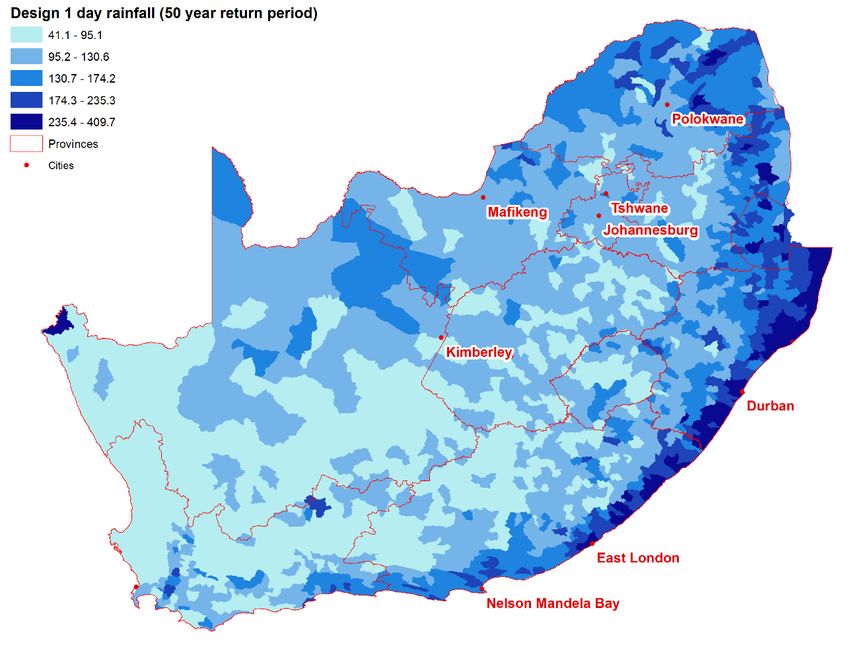
3.4 Flood exposure

We used vertical overland flow distance to the channel network as a proxy for the flood
exposure. Vertical overland flow distance is based on vertical distance between cell elevations
and the elevations calculated for the channel network in that cell. So, non-channel cells will
be assigned a value which represents the elevation difference between those cells and the
elevation of the nearest channel. The distance is expressed in the same units as the heights
and cell size values from the DEM grid which, in this case was metres. The vertical overland
flow distance was calculated using the open source SAGA GIS software (Olaya, 2004) based
on the inputs of the 30 m DEM and channel network information derived from the SCIMAP
model outputs. Using the extract by attribute function in the spatial analyst tool in ArcGIS,
areas with an elevation different of ≤10 m were extracted. Zonal statistics were run on the
extracted layers to determine the sum of the areas with a vertical overland distance of less or
equal to 10 m for each settlement. The resulting values were then divided by the total area of
the settlement and then multiplied by 100 to derive the percentage of each settlement situated
≤10 m above the nearest river channel. The output was then intersected with the National
Land Cover 2013-14 (GTI, 2015) to determine the land cover types present in the areas ≤10
m above the channel network and thus potentially exposed to floods.

4 RESULTS

4.1 Climate and hydrological characteristics

The 50-year return period daily rainfall as used in the flood hazard modelling shows an
interesting distribution across South Africa (Figure 3). It is however important to look at the
general patterns rather than the individual catchments because the values are based on
weather station observations and are strongly influenced by the length of the observed
records, location and density of the weather stations. This is especially true in the western
interior where there are very few weather stations.

The data show that the 50-year interval one day design rainfall is between 40 and 95 mm
across the whole of South Africa, Lesotho and Swaziland, with about 33% of the total area
falling in this class (Figure 2). Nearly 42% would get between 95 and 131 mm, 17% between
131 and 174 mm, and about 8% more than 174 mm. The highest values occur primarily along

 21

the eastern coast of South Africa, from East London through to the Mozambique border, well
as in parts of Mpumalanga and Limpopo, but also at various locations in the interior. So, most
of the eastern part of the country can expect to have more than 130 mm, and parts more than
230 mm of rainfall in a single day about once every 50 years. This is a considerable volume
of water as 130 mm equates to 1 300 m3/ha and, if this falls on a 10 000 ha catchment, it
would amount to 130 million m3 of water, enough to fill a large dam. To put this in perspective,
only 15% of South Africa’s dams have a capacity of 100 million m3 or more. However, please
note that some of the rainfall is likely to be absorbed by the soil or captured behind dams, so
the daily rainfall cannot simply be converted to a flood volume. The volume calculated above
just gives an indication. However, if the rainfall intensity is high (say >20 mm per hour) then
most of that rainfall will become floodwater because the soils and other permeable surfaces
simply cannot absorb that amount of water. If the soils were already moist or wet due to some
previous and recent rainfall, or if the high rainfall continues for many hours or days, then most
of the rainfall will become flood water.

Figure 2: 50-year return period design on day (daily) rainfall for South Africa (Schulze et al., 2008). The class intervals
 are based on a geometric scale to reduce the influence of extreme values

Another way to assess the rainfall-related flood hazard is to use modelled river flows which
are based on the rainfall records, other climatic inputs and biophysical characteristics of the
catchments. This modelling incorporates a number of factors that will determine how an area
of land responds to rainfall (Schulze et al., 2008; Smithers and Schulze, 2003). For example

 22

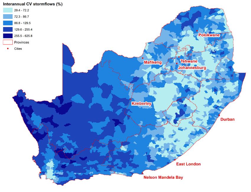
it can include estimates of the ability of the soils to absorb that rainfall as the rainfall event
progresses and so gives an idea of the flood volumes that can be expected. This assessment
shows that the high stormflows mainly occur in the eastern half of the region, but also in the
southern parts from Mossel Bay to Nelson Mandela Bay, and in the Boland and Groot
Winterhoek Mountains (Figure 3).

Figure 3: The modelled highest daily stormflow in a 10 year period (Schulze et al., 2008). The class intervals are based
 on a geometric scale to reduce the influence of extreme values.

This map makes it clear that settlements in the eastern part of South Africa, or Lesotho and
Swaziland, can expect high stormflows, especially those near the coast in the Eastern Cape,
in most of KwaZulu-Natal, in the Boland and the Garden Route. The variability between years
in the stormflows highlights an important characteristic of the rainfall, and thus the stormflows
in the western part of South Africa, namely its very high variability between years (Figure 4).
The map shows that while the highest stormflow in 10 years may be low in the western interior,
the variability is high and indicates that sudden floods are still possible, albeit very infrequently,
probably at recurrence intervals greater than 1 in 50 years. There are examples of these
periodic floods on record, driven by intense rainfall and triggering flash floods in the ephemeral
rivers which drain these landscapes because these arid landscapes cannot absorb the
rainwater. Some, such as the Laingsburg floods, get into the news but most have little impact
on settlements and are probably not reported. Conversely, all the areas that get relatively

 23

reliable and high rainfall every year, show a low variability between years such as the Boland
Mountains and parts of the Eastern Cape, KwaZulu-Natal and the Free State but the north-
eastern Free State has high variability. Some of the drier parts of Lesotho and Maputaland
also have high variability in their stormflows. The class intervals are based on a geometric
scale to reduce the influence of extreme values.

Figure 4: The variability in the stormflow between years (inter-annual) as a percentage of the mean stormflow (i.e. the
 Coefficient of Variation as a percentage) (Schulze et al., 2008).

Another useful measure of the flood risk is based on the observed floods and the ratio of the
flood discharge (m3/sec) to the normal mean annual discharge, also known as the K-ratio
(Kovács, 1988; Smithers, 2012). Essentially the K-ratio estimates how many times greater the
flood peak is than the typical river flow and it has been estimated for South Africa, Lesotho
and Swaziland, albeit some time ago (Kovács, 1988). The distribution of the ratio across the
region shows some similarities with the design rainfall and flood information summarised
above, with higher values found in the catchments in the southern and eastern parts and lower
values in the western interior (Error! Reference source not found.5). The highest ratios were
ound in the coastal catchments from Nelson Mandela Bay through to north of Durban K-ratio
= 5.4) with northern KwaZulu-Natal the highest at 5.6.

 24

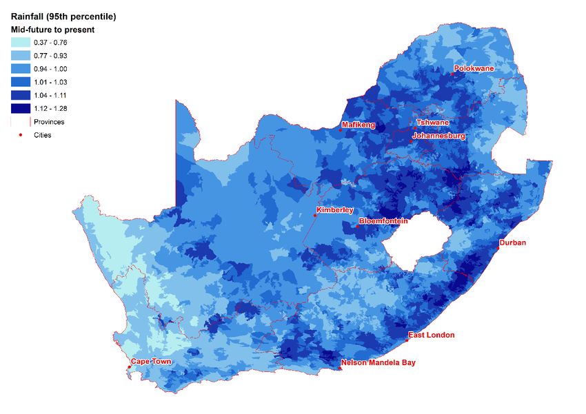
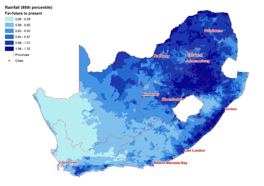
Figure 5: The regionalised K-ratio i.e. the ratio of the flood peak in m3/sec to the average annual flow in m3/sec for
 catchments in South Africa, Lesotho and Swaziland (Kovács, 1988). Digital version supplied by the Aurecon Group
 (Andre Görgens personal comm)

4.2 Projected increases in extreme daily rainfall

Although there are uncertainties about the changes in rainfall under future climates with
different models and different emission scenarios having different outcomes, there is general
agreement that rainfall intensities (the amount of rainfall in a given period of time) will increase.
So, under future climates it is likely that the design rainfall (Figure 2) will increase and that the
volumes of storm runoff will increase, leading to increased occurrence of floods. One way of
assessing the degree of the change is to compare future rainfall extremes (e.g. 95th percentile
of daily rainfall) with those under the current rainfall (1971-2000) based on the global climate
model outputs. This comparison indicates that in the near-future (2021- 2050) the extreme
daily rainfall will increase in many parts of the country, particularly over the Highveld and
northern Drakensberg, and in a broad belt along the south-eastern and eastern coast (Figure
6). The western and south-western regions are likely to experience a decrease, including the
winter rainfall region. This is consistent with an expectation that increasing temperatures will

 25

increase the intensity of the convection rainfall systems (e.g. thunderstorms) which are
characteristic of this part of the country (Dedekind et al., 2016).

Figure 6: The mean ratio of the near-future (2021-2050) and current (1971-2000) extreme daily rainfall (95th percentiles)
 for each quinary catchment. Values greater than 1.0 indicate an increase in the extreme daily rainfall.

In the far future (2070-2099) the same general pattern is evident with increases in the extreme
daily rainfall in the central, eastern and northern parts of the country and decreases in the
west and south-western parts, except for the coastal Agulhas to George area where there will
be an increase (Figure 7). Given the flooding and extensive flood damage caused in Gauteng
and parts of the adjacent provinces in recent years, these projections suggest that investment
is needed to mitigate and adapt to these conditions. This will include investment in restoring
ecological infrastructure, upgrading built infrastructure in combination with green infrastructure
(e.g. water sensitive urban design) and ensuring that settlements and infrastructure are
removed from high flood risk areas.

 26

Figure 7: The mean ratio of the near-future (2070-2099) and current (1971-2000) extreme daily rainfall (95th percentiles)
 for each quinary catchment. Values greater than 1.0 indicate an increase in the extreme daily rainfall.

4.3 Flood Hazard Index

The Flood Hazard Index (FHI), which is based on the catchment characteristics and design
rainfall, was averaged at the quinary catchment level and the classes were defined using the
standard deviations as the distribution of the FHI values followed a normal distribution.

Two catchment areas are shown in detail to illustrate the outputs of the model. The first shows
the quinary sub-catchments in the primary catchment U which includes all the river systems
between the Mtentweni River, north of Port Shepstone, and the Zinkwazi River, just south of
the Tugela (Figure 8). A very high FHI is found in the headwaters of the uMlazi River just south
of Pietermaritzburg and forms part of a band of high FHI which runs from north to south in this
catchment. The upper catchment of the Lovu River in the Drakensberg foothills also has an
area of high FHI. The lowest FHI values are found in catchments on the southern boundary
and low values are found along the coast north and south of Durban.

 27

Figure 8: The Flood Hazard Index calculated by the SCIMAP model for the primary catchment area U showing the
mean values per quinary catchment. Class intervals based on the standard deviation of the mean values per quinary
 catchment.

In the case of the Inkomati catchment, the very high FHI hazard is found at several points in
the valley of the Crocodile River, particularly to the east of KaNyamazane. A large portion of
the Crocodile River catchment also has a high FHI. There is also a relatively high FHI in the
Lowveld in the eastern part of the catchment, much of which is within the Kruger National Park
(Figure 9). The Highveld in the upper Komati catchment has a low to very low FHI, as do areas
in the north of this catchment. The white area in the south of the catchment is a portion of
Swaziland, which was not included in this study.

 28

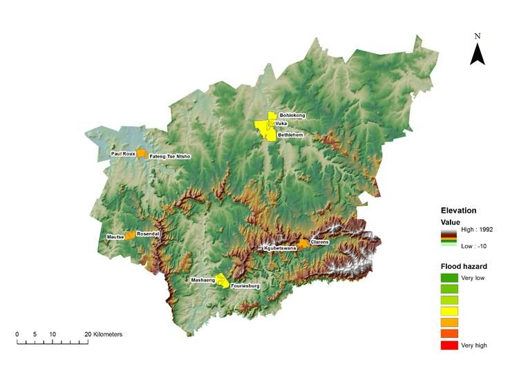
Figure 9: The mean flood hazard calculated by the SCIMAP model for the primary catchment area X (Inkomati River
System) for each quinary. Class intervals based on the standard deviation of the mean values per quinary catchment.

When assessed at the national level, the FHI is rated medium for much of the country, with
Namaqualand, the Kalahari, parts of the Karoo, the Limpopo valley and the Zululand coast
having a low to very low FHI (Figure 10). Very high FHI values are found in:
  The Sneeuberge north and west of Cradock in the catchments of the Pauls,
 Wilgerboom and Kwaai Rivers – all tributaries of the Great Fish River
  The Mbhashe River valley near Bashee Bridge
  A region of the Eastern Cape extending from the central Thina and Mzimvubu River
 valleys (south-east of Mount Frere) through to Donnybrook in KwaZulu-Natal
  The uMlazi River valley
  The central Tugela River valley, the uMfolozi near Ulundi
  The Drakensberg escarpment where it crosses the Crocodile and Olifants River
 valleys, and
  The Soutpansberg.

The FHI for the Cape mountains is generally relatively low at the national level, but there are
areas with a higher FHI in these mountains. The small portion of the Richtersveld estimated
to be very high FHI largely because it is mountainous and the land cover is predominantly
bare ground, but it is essentially uninhabited, giving it a low flood risk.

 29