The Effect of Income on Vehicle Demand: Evidence from China's New Vehicle Market - Joshua Linn and Chang Shen - Working Paper 21-17 June 2021 ...
←
→
Page content transcription
If your browser does not render page correctly, please read the page content below
The Effect of Income on
Vehicle Demand: Evidence
from China’s New Vehicle
Market
Joshua Linn and Chang Shen

Working Paper 21-17
June 2021
About the Authors
Joshua Linn is an associate professor in the Department of Agricultural and Resource
Economics at the University of Maryland and a senior fellow at RFF. His research
centers on the effects of environmental policies and economic incentives for new
technologies in the transportation, electricity, and industrial sectors. His transportation
research assesses passenger vehicle taxation and fuel economy standards in the
United States and Europe. He has examined the effects of Beijing’s vehicle ownership
restrictions on travel behavior, labor supply, and fertility.

Prior to joining RFF in 2010, Linn was an assistant professor in the economics
department at the University of Illinois at Chicago and a research scientist at MIT. He
was a senior economist at the Council of Economic Advisers from 2014–2015. He is
serving on a National Academies of Sciences, Engineering, and Medicine committee on
light-duty fuel economy. He is a co-editor for the Journal of Environmental Economics
and Management.

Chang Shen is a transportation economist with five years of research experience
investigating environmental issues in the transportation sector. Her research focuses
foremost on estimating consumers’ vehicle and travel demand, as well as evaluating
policies and market incentives in promoting greener transportation and reducing GHG
emissions. She holds a Ph.D. degree in Agricultural and Resource Economics (AREC)
from University of Maryland.
About RFF
Resources for the Future (RFF) is an independent, nonprofit research institution in
Washington, DC. Its mission is to improve environmental, energy, and natural resource
decisions through impartial economic research and policy engagement. RFF is
committed to being the most widely trusted source of research insights and policy
solutions leading to a healthy environment and a thriving economy.

Working papers are research materials circulated by their authors for purposes of
information and discussion. They have not necessarily undergone formal peer review.
The views expressed here are those of the individual authors and may differ from those
of other RFF experts, its officers, or its directors.

Sharing Our Work
Our work is available for sharing and adaptation under an Attribution-
NonCommercial-NoDerivatives 4.0 International (CC BY-NC-ND 4.0) license. You
can copy and redistribute our material in any medium or format; you must give
appropriate credit, provide a link to the license, and indicate if changes were made,
and you may not apply additional restrictions. You may do so in any reasonable
manner, but not in any way that suggests the licensor endorses you or your use.
You may not use the material for commercial purposes. If you remix, transform, or
build upon the material, you may not distribute the modified material. For more
information, visit https://creativecommons.org/licenses/by-nc-nd/4.0/.
The Effect of Income on Vehicle Demand: Evidence
                   from China’s New Vehicle Market

                                          J OSHUA L INN

                                          C HANG S HEN*

                                              June 2021

                                               Abstract

             Growth of private vehicle ownership in low-income and emerging countries is
      a dominant factor in forecasts of global oil demand and greenhouse gas emissions.
      Countries such as China are expected to experience rapid income growth over the next
      few decades, but little causal evidence exists on its effect on car ownership in these
      countries. Using city-level data on new car sales and income from 2005 to 2017, and
      using export-led growth to isolate plausibly exogenous income variation, we estimate
      an elasticity of new car sales to income of about 2.5. This estimate indicates that recent
      projections of vehicle sales in China have understated actual sales by 36 percent and
      carbon dioxide emissions by 18 million metric tons in 2017. The results suggest that, to
      meet its climate objectives, China’s climate policies will need to be substantially more
      aggressive than previous forecasts indicate.

   * Linn:   University of Maryland and Resources for the Future (linn@umd.edu). Shen: University of
Maryland. The authors thank Anna Alberini, Jim Archsmith, Erich Battistin, Jing Cai, and Cinzia Cirilo for
helpful comments.

                                                    1
1 Introduction
Global oil consumption and greenhouse gas (GHG) emissions from transportation are
expected to increase over the next few decades, with lower-income countries causing most
of the growth. The US Energy Information Agency predicts that oil consumption and
transportation energy consumption will grow roughly 15 percent between 2020 and 2040.
OECD and non-OECD countries are expected to follow diverging paths: consumption
is expected to decline 3 percent for the former and increase nearly 30 percent for the
latter (EIA, 2019). Projections from the International Energy Agency and other major
organizations are broadly similar.
China is a major driver of these diverging trends. China’s oil consumption is expected
to grow 20 percent between 2020 and 2040 (EIA, 2017). Rising vehicle ownership explains
much of this growth—in both China and other non-OECD countries. China’s vehicle stock
is expected to grow by 200 million units between 2020 and 2040, accounting for nearly all
of the global growth in the vehicle stock (BloombergNEF, 2020).1
For China, and many other countries, climate policy depends crucially on these emis-
sions forecasts. For example, under the United Nations Paris Agreement, China has
pledged to peak its emissions by 2030 and then substantially reduce emissions. Total
transportation sector emissions, which account for 9 percent of China’s GHG emissions
(IEA, 2017), equal the emissions rate of vehicles multiplied by the number of vehicles
and miles traveled per vehicle. China’s transportation policies focus mostly on reducing
the new vehicle emissions rates and not the levels of emissions. Therefore, to achieve
the emissions target under the Paris Agreement the greater the future vehicle ownership
and use, the more China has to reduce vehicle emissions rates (Pan et al., 2018); if vehicle
ownership turns out to be 10 percent higher than expected, policies would have to reduce
emissions rates by an additional 10 percent. Globally, countries rely almost exclusively
on GHG emissions rate standards for passenger vehicles to reduce transportation sector
emissions, and similar policy uncertainty applies to these countries.
Unfortunately, assumptions behind these forecasts rest on little empirical support. In
the computational models that generate the forecasts, oil consumption and GHG emissions
from passenger vehicles are closely linked to household vehicle ownership. An extensive
literature correlates income with vehicle ownership in the United States, Europe, and
other OECD countries (Dargay, 2001; Dargay, Gately, and Sommer, 2007; Nolan, 2010;
1 Thesituation is comparable to that for anticipated growth in electricity consumption, where growth is
concentrated among non-OECD countries and driven largely by uptake of energy-consuming durable goods,
such as refrigerators and air conditioners (Auffhammer and Wolfram, 2014; Davis, Fuchs, and Gertler, 2014).
2Blumenberg and Pierce, 2012; Oakil, Manting, and Nijland, 2018). Most projections of
future vehicle ownership in China and other non-OECD countries from the past two
decades rely on the assumption that ownership and use will follow patterns observed in
other countries. For example, Huo et al. (2007) forecast vehicle ownership in China using
data from in Europe, Japan, and other countries, assuming that the effect of GDP per capita
will be the same in China. He et al. (2005) and Yan and Crookes (2009) use similar methods,
as do forecasts from organizations such as the International Energy Agency, which receive
a lot of attention from policymakers. However, Wang, Teter, and Sperling (2011) argue that
periods of early motorization in the United States and Europe may be more relevant to
future motorization in China; in that case, basing projections on recent OECD data could
yield overly conservative estimates of China’s future oil consumption and GHG emissions.
Recently, income and vehicle ownership have exploded in China, with average income
per capita growing 11.9 times and new vehicle sales growing 7.6 times between 2000 and
2017 (CEIC Data). This situation presents an opportunity to evaluate the assumptions that
underlie the projections of future vehicle ownership and GHG emissions in China. That is,
have recent projections of vehicle ownership in China proven to be accurate?
We estimate the recent relationship between income and new car ownership in China
and compare the results with recent forecasts of vehicle ownership. The main data include
total new vehicle sales, income, and other socioeconomic variables by city and year for
2005–2017. This period includes 9.6 percent annual growth in income and 20 percent annual
growth in new vehicle sales. During these years, sales grew from 5.8 to 29 million units, as
China became the world’s largest new car market, roughly twice as large as markets in the
United States or Europe.
The objective is to estimate the causal effect of income on car ownership, and a major
challenge is that income is endogenous to car ownership due to reverse causality and
omitted variables. For example, if vehicle ownership reduces travel costs and allows people
to find better jobs, reverse causality could exist from ownership to income. Omitted factors
that may be correlated with income and also affect car ownership, such as cultural trends
related to car ownership, would cause omitted variables bias. Besides being potentially
endogenous, city-level income may be measured with error.
We adopt an instrumental variables strategy to address the endogeneity and measure-
ment error. We employ a Bartik-style instrumental variable (IV) that is the interaction of a
city’s education employment in 2004 with China’s annual high-technology exports. The
relevance of the instrument is supported by a) high-technology exports having driven
much of China’s economic growth over the past two decades; and b) cities with high
initial education employment having large skilled worker populations who can produce
3high-technology exports. The exclusion restriction is that 2004 education employment is
uncorrelated with subsequent unobserved factors that affect vehicle ownership via chan-
nels other than income. We provide evidence supporting this assumption, including a lack
of correlation between 2004 education employment and subsequent shocks to other drivers
of vehicle ownership, such as the quality of public transportation.
We find that a 1 percent increase in income causes total new vehicle sales to increase by
2.5 percent. Income does not affect the sales-weighted average price of new vehicles sold,
meaning that as income has grown, sales of low- and high-price vehicles have grown by the
same proportion. Likewise, the elasticity of new vehicle sales to income does not appear
to be correlated with a city’s initial income, again suggesting proportional growth. The
estimate is robust to alternative functional forms and controlling for other socioeconomic
variables.
Comparing our results with the literature, we conclude that recent projections of future
new vehicle sales in China may be vastly understated. Our estimates mean that in 2017,
rising income increased sales by about 36 percent and increased carbon dioxide emissions
by about 18 million metric tons more than predicted by recent forecasts. In the long run,
annual sales are proportional to the new vehicle stock, suggesting that recent forecasts
of new vehicle sales underpredict the effect of rising income on emissions by roughly 26
percent. Our results indicate that recent forecasts may substantially underestimate China’s
future oil consumption and GHG emissions. This implies that China will need to adopt
more aggressive climate policies to meet its GHG targets.
We contribute to several literature strands. First, several studies project China’s future
vehicle stock. A typical method is to assume that vehicle ownership is an S-shaped function
of per-capita gross domestic product (GDP). The rationale for this is that in OECD countries,
vehicle ownership increased slowly at low levels of GDP, rose steeply, and then leveled off
(Lu et al., 2018). For instance, Huo et al. (2007) assume the vehicle ownership rate follows
an S-shaped Gompertz function of per-capita GDP and conclude that the Chinese highway
vehicle stock will reach 389–495 million units by 2040. Huo and Wang (2012) compare
several S-shaped functional forms and account for income inequality and vehicle prices.
Lu et al. (2018) and Gan et al. (2020) use similar methods and more recent data, projecting
that China’s vehicle stock will reach 400–600 million units by 2050.
These forecasts assume parameters for the function linking vehicle stock to income,
including a saturation rate. Most previous studies assume saturation rates of 200–800 cars
per thousand people (He et al., 2005; Dargay, Gately, and Sommer, 2007; Huo et al., 2007;
Huo and Wang, 2012; Lu et al., 2018), which is based on observations from other countries.
Gan et al. (2020) comment that transferring parameters from other countries to China is
4arbitrary, and they use household survey data instead to calibrate their model.
In contrast to this literature, rather than calibrating a curve to data from other countries,
we use historical data from China to estimate the effect of income on total new vehicle
sales, accounting for the potential endogeneity of income. To our knowledge, ours is the
first study to investigate the effect of income at the city level. Nearly all prior research
estimates vehicle growth using national data. However, as we illustrate, Chinese cities have
had imbalanced development and it was a national strategy to prioritize the development
of certain regions (Shen, Teng, and Song, 2018). Each city also has its own preferences
for public transportation and road systems. Different cities might exhibit very different
vehicle growth patterns. Our balanced panel of city-level data allows us to exploit cross-
sectional and time-series variation of income and new car sales and consider whether the
income–sales relationship varies across cities.
We also contribute to the broader literature on income and energy-consuming durables
and future GHG and oil demand. As noted, little research exists on the effect of income on
new vehicle demand in non-OECD countries, although some research has been undertaken
on household appliances and residential energy-efficient and renewable energy products,
such as solar panels. McNeil and Letschert (2010) find that ownership of refrigerators,
washing machines, televisions, and air conditioners increases with household income,
urbanization, and electrification rates. They also document an S-shaped relationship
between income and appliance ownership. Auffhammer and Wolfram (2014) and Li
et al. (2019) report somewhat conflicting evidence on the relationship between income
and appliance ownership. Auffhammer and Wolfram (2014) show that the proportion of
households above the poverty line affects the uptake of energy-using durable goods in
rural China. However, Li et al. (2019) show that the income threshold for ownership is
correlated with the cost of the appliance. In contrast to Auffhammer and Wolfram (2014),
they find that changes in the income distribution have negligible effects on penetration rate
of household appliances.2
Closely connected to the literature on income and energy-consuming durables is the
extensive literature on the Environmental Kuznets Curve (EKC; for example, Shafik and
Bandyopadhyay, 1992; Dasgupta et al., 2002; Wagner, 2008; Yao, Zhang, and Zhang, 2019).
This literature examines the relationship between income (or GDP) and pollution, and
most studies use aggregate national or regional data. Many studies document an inverted
U-shaped relationship between income and emission: at low levels of income, emissions
rise with income, but at high levels of income, emissions decline with income. However,
2Avast literature exists on income and appliance ownership in OECD countries, such as Zhao et al. (2012)
and Mundaca and Samahita (2020).
5studies disagree on the factors explaining this relationship (Kaika and Zervas, 2013); many
argue that in the early stages of economic development, economic expansion is fuelled
by heavy and polluting industry. Subsequently, the economy shifts from heavy industry
to services and environmental regulation strengthens, causing pollution to decline. Yin,
Zheng, and Chen (2015) confirm an inverted U-shaped relationship between per-capita
income and carbon dioxide emissions in China.
Our analysis contributes to the EKC literature in two main ways. First, ours is among
the small number of papers that addresses the endogeneity of income to other factors that
affect pollution, such as road networks and public transportation. Second, we demonstrate
that income can affect pollution through microlevel household behavior, which contrasts
with the predominant use of macrolevel data in the EKC literature.
Finally, the literature on long-run climate policy using integrated assessment models
(IAMs) and other aggregate models calibrates the relationship between GDP and emissions
absent policy intervention (Nordhaus and Yang, 1996; Cantore, 2011; Krey et al., 2012;
Vliet et al., 2012; Ruijven et al., 2012; Calvin et al., 2013; Steckel et al., 2013; Luderer et
al., 2015; Cherp et al., 2016; Calderón et al., 2016; Zwaan et al., 2018; Nieto et al., 2020).
These models can be used to estimate the efficient carbon price or the costs of achieving
long-run policy objectives, such as maintaining expected temperature changes below a
certain threshold. Often, IAMs are calibrated to forecasts of future GDP and emissions.
We find that at least for China, those forecasts may vastly understate future transportation
emissions. Given China’s contribution to global emissions, that would cause the forecasts
to understate global transportation emissions by a nontrivial amount—and by even more
if our results pertain to other non-OECD countries. Therefore, more accurate predictions
of future vehicle ownership in China and perhaps other non-OECD countries could have
implications for climate policy analysis in IAMs.
2 Data and Summary Statistics
We use data on new vehicle registrations in all of China from 2005 to 2017. The Chinese
Department of National Security collects the data, which contain information on the total
number of new vehicles registered by city, month, model, and usage purpose (personal
or business). The data include vehicle attributes, such as engine size and manufacturer
suggested retail price. Because we are interested in the effect of personal income on vehicle
ownership, we exclude business purchases. Imported cars are also excluded due to a lack
of price information (the results are similar if we include these, which account for a small
share of total registrations).
6We use counts of new vehicle registrations as proxies for vehicle sales. Tan, Xiao, and
Zhou (2019) compare the new vehicle registration data with statistics on vehicle sales from
the China Automotive Industry Yearbook and find that the registration data account for
70 percent of total vehicle sales. However, further investigation suggests that the sales
data, rather than the registration data, are misleading. Many agencies and organizations
in China compile their own sales statistics, such as the China Association of Automobile
Manufacturers, the State Information Center, and the Chinese Passenger Cars Association.
Each organization uses its own data collection methodology. For instance, the China
Association of Automobile Manufacturers includes unrealized orders from manufacturers.
In addition, most of these statistics rely on self-reported data from manufacturers. It is not
uncommon for vehicle manufactures to fake sales, and many automobile industry analysts
are turning to registration data. In the remainder of the paper, we use the terms sales and
registrations interchangeably.
One potential concern about using registration data is that consumers may not imme-
diately register their vehicles after purchase. In that case, registrations would lag sales.
However, the month of registration is a good proxy for the month of sales. Most Chinese
car buyers choose to pay an additional service fee and apply for registration through the car
dealers immediately after they complete their purchases. The application process usually
takes 2–7 days, and driving without a registration would add penalty points to the driver’s
license. Therefore, the registration month and purchase month are the same for the majority
of vehicles, and the two may differ by at most a month. This situation likely introduces
little measurement error because we aggregate the monthly data to the annual level.
We combine the registration data with a set of socioeconomic variables from the China
City Statistical Yearbook, which is published annually by the National Bureau of Statistics
of China (NBSC). Each year, NBSC distributes questionnaires to municipal statistics de-
partments. Province-level statistics departments and the NBSC check the validity of the
responses. For each city, the yearbook includes average income per capita, which is the
key independent variable in the econometric analysis; the built area (constructed areas for
residential, commercial, or industrial use); area of paved roads (road length multiplied by
width); population; number of buses and taxis in the public transportation system; total
retail revenue; and the share of education sector employment in total employment. We
also gather information on national-level high-technology exports from the World Bank,
which defines these as products with high R&D intensity, such as aerospace, computers,
pharmaceuticals, scientific instruments, and electrical machinery.
Table 1 summarizes the car registration and socioeconomic variables. The dataset
contains 3,627 unique city-year observations (a balanced panel of 279 cities over 13 years).
7New car expenditures and the number of cars sold are aggregated to the city-year level,
and average car price is weighted by the number of cars sold. Car sales and socioeconomic
variables vary substantially across cities.
Table 1: Summary statistics
Main variables mean std.dev coef. var. min max median
New cars sold (thousand units) 37.9 62.0 1.6 0.4 727.0 17.0
New car expenditure (billion RMB) 5.9 10.5 1.8 0.1 140.1 2.4
Car price (thousand RMB) 153.0 27.0 0.2 94.1 259.3 148.9
Income per capita (thousand RMB) 41.4 16.3 0.4 8.8 135.0 40.4
Built-up area (square km) 121.0 165.2 1.4 6.0 1446.0 70.0
Area of paved roads (square km) 15.9 21.7 1.4 0.4 214.9 8.4
Population (thousand people) 4,354.2 3,098.4 0.7 172.2 34,332.3 3,700.0
Buses (thousand units) 1.3 2.8 2.1 0.0 35.8 0.5
Taxis (thousand units) 3.1 6.0 2.0 0.1 68.5 1.5
Total retail expenditure (billion RMB) 73.0 111.0 1.5 1.6 1183.0 38.6
Employment percentage in education (2004) 4.8 4.5 0.9 0.1 41.6 3.9
National high-tech export (billion RMB) 3,786.0 590.2 0.2 2,461.6 4,509.9 4,001.6
Notes: The data contain 3,627 observations. "Built area" is the area of land constructed for residential,
commercial, or industrial use. "Bus" and "taxi" are the numbers of buses and taxis operating in the city. All
monetary variables are adjusted for inflation and measured in 2017 RMB. "Coef. var." is the coefficient of
variation.
Figure 1 illustrates income growth for five groups of cities between 2005 and 2017. We
compute quantiles of the distribution of city-level average income per capita using 2005
income data, and we assign each city to a quintile group. The figure shows the average
income of cities in each group, with average income normalized to 1 in 2005 to facilitate
comparison of income growth across cities. All five quintiles saw tremendous growth, as
well as a steady pattern of converging income levels across cities. Between 2005 and 2017,
the average income for cities in the lowest quantile grew by a factor of 3.64, indicating a
remarkable 28 percent average annual growth rate. In contrast, the average income for
cities in the highest quantile grew by a factor of 2.51. This convergence eliminated 67
percent of the difference between the average income of the fifth and first quantiles: in
2005, the average income of the highest quantile is 214 percent of the average of the lowest
quantile, whereas in 2017, this number decreased to 148 percent. The income growth and
variation across cities helps identify the effect of income on car ownership and facilitates
an analysis of whether the effect varies across cities.
8Figure 1: Income Growth by City Income Quintile
Notes: All cities are divided into five quintiles according to their income in the initial period (2005). For
each year, we calculate the average income of cities within each of the five quintiles. We normalize the
quintile-level averages by their 2005 values.
Table 2 provides further insight into the income dynamics during the study period.
Each column indicates a city’s 2005 income quintile, and each row indicates a city’s 2017
income quintile (based on the 2017 rather than the 2005 income distribution). Quintile 1
is the lowest, and Quintile 5 is the highest. Each cell reports the percentage of cities that
were in the indicated 2005 income quintile and that belong to the 2017 income quintile. For
example, 50 percent of cities in the lowest 2005 income quintile belong to the lowest 2017
income quintile, whereas 36 percent of cities in the lowest 2005 income quintile belong to
the second 2017 quintile. The table shows that many initially low-income cities catch up to
and pass many initially higher-income cities; for example, 15 percent of cities in the lowest
income quintile in 2005 belong to the top three quintiles in 2017.
The next two figures present summary statistics about new car registrations and at-
tributes. All monetary values are converted to 2017 RMB using the annual consumer price
index. Figure 2 reports the growth rate of vehicle sales (panel a) and revenue (panel b) by
income quintile, with quintiles defined as in Figure 1 and 2005 levels normalized to 1 for
comparability across quintiles. Total sales and expenditure have a similar pattern to income
growth from Figure 1, with sales and revenue increasing more quickly in low-income cities
than in high-income cities. The similarity of the patterns across the two figures previews
our main finding of a strong connection between income and new car demand; in fact,
panel (d) shows that registrations outpaced income growth for each group of cities.
9Table 2: Quintile Switching
2005 income level
1 2 3 4 5
1 (lowest) 50 % 30 % 13 % 5% 2%
2 36 % 23 % 27 % 14 % 0%
2017 income level 3 9% 29 % 27 % 25 % 11 %
4 4% 16 % 32 % 30 % 18 %
5 (highest) 2% 2% 2% 25 % 69 %
Notes: Each column indicates a city’s 2005 income quintile, and each row indicates a city’s 2017 income
quintile (based on the 2017 rather than the 2005 income distribution). Each cell reports the percentage of
cities that were in the indicated 2005 income quintile and that belong to the 2017 income quintile.
Panel (c) shows that the average real new car price has been declining during this
period, indicating that although the aggregate demand for new cars increased, households
are not systematically buying more expensive cars at the end of the period relative to what
they were buying at the beginning. This is consistent with domestic car manufacturing
evolving during the sample, with most domestic brands targeting low- and middle-price
vehicles, putting downward pressure on average prices.
10Figure 2: Growth of Sales, Expenditure, and Price by Income Quintile
(a) Sales (b) Expenditure
(c) Average price (d) Expenditure share in income
Notes: All monetary values are converted to 2017 RMB using the annual CPI.
The average new car price declined between 2008 and 2016. During this period, income
growth slowed and vehicle policies changed. From January through December 2009 and
October 2015 through December 2016, China reduced purchase taxes from 10 percent
to 5 percent for cars with small engines. The change likely increased demand for such
cars, which also tend to be less expensive than cars with large engines. Moreover, in
2008, China introduced a fuel economy standard that required a 10 percent reduction in
fuel consumption rates (the fuel consumption rate, measured in liters per kilometer, is
the inverse of fuel economy, in miles per gallon). Manufacturers attempted to meet this
standard by incentivizing consumers to purchase cars with low fuel consumption rates,
11which also tend to have low purchase prices. Panel (b) shows that fuel consumption rates
increased from 2005 through 2008 but declined after 2008, as the fuel economy standards
tightened.
Panels (c) and (d) show that average horsepower and weight increased over the sample
period at similar rates across quintiles. The overall upward trends are interrupted by
temporary decreases in 2008 and 2016, which coincide with the engine tax policy changes.
Overall, the data show dramatic growth of new vehicle sales and income. The rates
varied considerably across cities, with income and sales converging over time. Average
prices decreased between 2005 and 2017, and much of the decrease coincided with tax policy
changes and fuel economy regulation. The empirical strategy controls for the policies.
Figure 3: Average Vehicle Attributes by Income Quintile
(a) Engine size (b) Fuel consumption rate
(c) Horsepower (d) Gross weight
123 Empirical Strategy
The first subsection provides a theoretical framework that yields the estimating equation;
the second subsection discusses the IV estimation that accounts for the endogeneity of
income.
3.1. Economic Framework and Estimating Equation
We motivate the estimating equation by examining a framework that links income to
new car ownership. For an individual household, purchasing a new car would increase
the household’s utility because of the comfort and convenience of travel. For example,
suppose a household member commutes by public transportation and purchasing a car
would reduce commuting time. The car may also allow household members to take new
trips. Besides comfort and convenience, owning a car may confer status to the household.
When deciding whether to purchase the car, the household compares the benefit of
ownership with the costs. The costs include the purchase price (the forgone consumption
of other goods), fuel costs, and maintenance. If car ownership is a normal good, it increases
with income. If we aggregate across households, total new car sales increase with income.3
The objective is to estimate the causal effect of household income on new vehicle
purchases and expenditure, conditional on other factors that could affect new car demand.
Because population determines the size of the potential market for new vehicles, it is
natural to begin by assuming that car purchases and expenditure are proportional to
income conditional on population, giving rise to the following regression:
lnYjt = α N lnNjt + α P lnPjt + X jt δ + γ j + τt + e jt (1)
The dependent variable is the log of either new vehicle purchases or expenditure in city
j and year t. The variable Njt is income, Pjt is population, X jt is a vector of controls, γ j
includes city fixed effects, τt includes year fixed effects, and e jt is an error term. Note that
instead of controlling for the log of population, we could normalize the dependent variable
and income by population. Normalizing by income would amount to setting α P equal to
-1. Because equation (1) allows the coefficient to differ from -1, this specification is more
flexible.
3 Thisstatement could be formalized by considering a model in which a household derives utility from a
car and a composite good. The utility from car ownership depends on its attributes (such as interior space
or performance) and an idiosyncratic preference shock. If the utility function exhibits decreasing marginal
utility for the composite good, an increase in income raises the probability that the household purchases the
car. Aggregating across households, we conclude that total new car sales increase with average income.
13The vector X jt includes factors that may affect new car demand independently of
income, such as the built-up area in the city (constructed area for residential, commercial
or industrial use), area of paved roads, population, number of buses and taxis in the
city’s public transportation system, and total retail revenue (that is, a proxy for retail
expenditures). The city fixed effects control for time-invariant attributes, such as geographic
proximity to other cities (which could affect travel demand), and the year fixed effects
control for aggregate shocks that affect car sales proportionately, such as tax incentives.
The main coefficient of interest in equation (1) is α N . Because the dependent variable
and income enter the equation in logs, the coefficient is interpreted as an elasticity; a
coefficient of 1 means that a 1 percent increase in income is associated with a 1 percent
increase in car purchases or expenditure. We expect α N to be positive because an increase
in income raises new vehicle demand.
We consider the log-log relationship between average city income and sales to be an
approximation of a potentially more complex relationship. For example, sales could be a
function of the household income distribution if a threshold level of income exists below
which households do not purchase new vehicles. As the household income distribution
shifts to the right over time, sales increase but the relationship between average city income
and total sales may not be iso-elastic. We show that we use the log-log approximation
because it appears to fit the data reasonably well.
Note that we do not model explicitly the effects of vehicle attributes on household
purchase decisions, as we might if we were to estimate a discrete choice model rather than
the reduced-form equation (1). We choose the reduced-form approach because a discrete
choice model is not necessary given the scope of our paper; implementing it introduces
unnecessary structure and the need to instrument for endogenous vehicle attributes, such
as vehicle price. In equation (1), the log income coefficient (α N ) includes the mediating
effects of vehicle attribute changes caused by income changes. The next subsection explains
our approach to controlling for attribute changes that are not caused by income changes,
such as the vehicle regulations that affect fuel economy and engine size discussed in the
previous section.
3.2. IV Estimation and Interpretation
The theoretical framework at the beginning of the previous subsection indicates three
reasons why estimating equation (1) by ordinary least squares (OLS) would yield incon-
sistent estimates of α N : reverse causality, omitted variables bias, and measurement error.
Reverse causality could arise if owning a car reduces commuting costs, expanding an
14individual’s job opportunities and income from employment.
Omitted variables bias could occur if variables other than income affect the costs and
benefits of owning a car. We mentioned the quality of transportation as one example, and
many others exist, such as vehicle operating and maintenance costs. Although we attempt
to control for variables that affect new car demand independently of income, such as the
number of buses and taxis operating in a city, many such variables are unobservable or
difficult to measure, such as the quality of public transportation.
Finally, income may be measured with error. We use the average income of a city’s
population, but the relevant measure may be the income of households considering buying
new vehicles. Note that a city’s average income and the average income of potential new
car buyers are likely to be highly correlated with one another, but using average citywide
income likely introduces some measurement error.
Given these concerns, we use a Bartik-style instrument based on high-technology export-
driven income growth. A classic Bartik instrument is formed by interacting local industry
shares and national industry growth rates. It is commonly used across many fields in
economics, including labor, public, development, macroeconomics, international trade,
and finance (Goldsmith-Pinkham, Sorkin, and Swift, 2020; Beaudry, Green, and Sand, 2012;
Nunn and Qian, 2014; Baum-Snow and Ferreira, 2015; Jaeger, Ruist, and Stuhler, 2018).
The literature on export-driven income growth motivates the IV, which is the interaction
of national high-technology exports with the city’s 2004 education sector employment. We
use high-technology exports defined by the World Bank, which include products with
high R&D intensity in aerospace, computers, pharmaceuticals, scientific instruments, and
electrical machinery. Numerous studies find that high-technology exports have substan-
tially improved economic growth. For instance, Hausmann, Hwang, and Rodrik (2007)
show that export quality is positively correlated with growth, and Falk (2009) shows that
high-technology exports have a positive effect on economic growth in OECD countries.
Jarreau and Poncet (2012) confirm that high-technology exports promote economic growth
in China. They exploit variation in export sophistication at the province and prefecture
levels and find that regions specializing in more sophisticated goods subsequently grow
faster.
Moreover, human capital growth has contributed to high-technology exports (Stokey,
1991; Levin and Raut, 1997; Mehrara, Seijani, and Karsalari, 2017; Mulliqi, Adnett, and
Hisarciklilar, 2019). Thus, the literature documents a strong connection from human capital
growth to high-technology export growth to income growth. Given these findings, we
specify the first stage as
15lnNjt = β X ln( Et ) · Hj + β P lnPjt + X jt η + γ j + τt + µ jt (2)
where Et is national high-technology exports and Hj is the city’s education employment in
2005. The second stage is
lnYjt = α N lnN
djt + α P lnPjt + X jt δ + γ j + τt + e jt (3)
The IV specification is similar to equation (1), except that we use a Bartik-style instrument
for income. The aforementioned literature on export-driven economic growth establishes
the relevance of the instrument. We show that the instrument is a strong predictor of
income, reducing potential concern about weak instruments bias. Moreover, using pre-
sample education employment and aggregate exports addresses potential concerns about
reverse causality and omitted variables bias. Specifically, it eliminates reverse causality
because city-level new vehicle purchases cannot plausibly affect a city’s 2004 education
employment. Moreover, the IV reduces the likelihood that changes in a city’s predicted
(second-stage) income are correlated with other factors affecting demand for cars, such as
public transportation.
The IV reduces measurement error because export-driven high-income growth likely
affected workers with high human capital, who are more likely than other workers to
purchase new cars. That is, if we were using an instrument based on income to low-skilled
or agricultural workers, who purchased relatively few cars, we might be exacerbating
rather than reducing measurement error.
The exclusion restriction is that a city’s 2004 educational employment is uncorrelated
with factors that subsequently affect new car sales independently of income and are not
included in the IV estimation. Omitted variables correlated with the instrument are likely
the most important remaining concern about the IV strategy. Although unobserved factors
may be correlated with initial employment, we show that the city’s 2004 educational
employment is uncorrelated with 2004 levels and 2004–2017 growth of variables that may
affect car ownership independently of income, such as road space, built area, and the
number of buses and taxis. That observed factors are uncorrelated with initial employment
supports the exclusion restriction, but that restriction cannot be tested directly.
Care must be taken when interpreting the IV coefficient in equation (1). It identifies
the effect of income driven by expanding exports and includes effects of income mediated
through other factors that are not included in the estimation. For example, if rising income
makes owning a new car more fashionable, the IV coefficient includes that effect.
As another example, consider traffic congestion. If rising income increases driving
16and raises congestion, the coefficient includes that (presumably negative) effect of traffic
congestion. If congestion increases for reasons besides income, the IV estimate would be
consistent as long as the instrument is uncorrelated with the initial congestion level.
A similar argument pertains to other factors affecting car demand, such as public
transportation quality and vehicle attribute changes. If rising income causes cities to invest
more in public transportation, reducing demand for cars, the IV estimate would capture
the effect of income on car sales, net of the opposing effect of public transportation quality.
Likewise, the IV estimate includes vehicle attribute changes caused by increasing demand
for new cars. At the same time, the IV strategy controls for the effects of other factors
on vehicle attributes, such as fuel economy regulation, to the extent that these factors are
uncorrelated with the IV.
Before turning to the estimation results, we comment on dynamics. We have assumed a
contemporaneous relationship between income and new car sales. However, new car sales
could respond to lagged income or a moving average of recent income if household-level
income shocks are transitory. We allow for such possibilities in the robustness analysis.
4 Results
This section reports the main results and robustness analysis and compares our esti-
mates with recent forecasts of new vehicle sales in China.
4.1. Main Results
Table 3 reports estimates of equation (1) (OLS) and equation (3) (IV). Column 1 shows
the OLS estimate of the key coefficient, α N , from equation (1). The specification includes
city fixed effects, year fixed effects, and province by year interactions. Standard errors
are reported in parentheses, clustered by city. The coefficient on log income is 0.73 and
statistically significant at the 1 percent level. The estimate means that a 1 percent increase
in income is associated with a 0.73 percent increase in new car sales.
As the previous section mentioned, the OLS estimate of α N is likely to be inconsistent
because of reverse causality, omitted variables bias, and measurement error. Column
2 of Table 3 reports the IV coefficient, using the interaction of the city’s 2004 education
employment with aggregate high-technology exports in the corresponding year. The IV
estimate is 2.53, which is significant at the 1 percent level.
The IV coefficient is about three times greater than the OLS coefficient in column
1, which could be explained by reverse causality, omitted variables that are negatively
17Table 3: Effect of Income on Vehicle Registrations, Expenditure, and Average Price
(1) (2) (3) (4) (5) (6)
Log new Log new Log Log new Log new Log average
Dependent var:
registrations registrations income registrations expenditure price
Estimated by: OLS IV OLS IV IV IV
Log income 0.73 2.53 2.07 2.64 0.10
(0.11) (0.39) (0.52) (0.40) (0.08)
Log income * post 2010 -0.50
(0.32)
Log income instrument 2.29
(0.25)
Observations 3,627 3,627 3,627 3,627 3,627 3,627
Effective F stat for IV 83.33 83.33 22.88 83.33 83.33
Kleibergen-Paap stat 44.95 44.95 40.36 44.95 44.95
Underidentification p val 0.00 0.00 0.00 0.00 0.00
Notes: The table reports coefficient estimates with standard errors in parentheses, clustered by city. Column
headings state the dependent variable and estimation method. All regressions include city fixed effects, year
fixed effects, and province–year interactions.
correlated with income, or measurement error that causes attenuation bias. We return to
the economic interpretation of this estimate at the end of this section. Column 3 shows the
first-stage coefficient on the instrument, which is precisely estimated. Column 2 shows that
the first-stage effective F-statistic is 83, reducing concerns about weak instruments bias.4
Column 4 allows for different effects of income on registrations for two periods:
2005–2010 (particularly high income growth) and 2011–2017 (slower income growth).
The negative coefficient on the interaction term indicates that income had a smaller effect
in the latter period, although the estimate is not statistically significant, and it indicates just
a 25 percent decline in the elasticity across the two periods.
Having shown that rising income causes total new registrations to increase, we consider
how income affects the total expenditure on new vehicles and average prices. Columns 5
and 6 are the same as column 2, except that the dependent variable is the log of new car
expenditures (column 5) or the log of the sales-weighted average price (column 6). The
income coefficient in column 5 is similar to that in column 2, indicating that an increase in
income causes new car registrations and expenditures to increase by the same proportion.
Consistent with that result is that the coefficient in column 6 is small and not statistically
4 We use effective F statistics developed by Olea and Pflueger (2013) for detecting weak instruments. The
approach is robust to heteroskedasticity, time series autocorrelation, and clustering, which are likely to occur
in our data. However, it is only available for settings with one endogenous regressor; we are not aware of a
heteroskedasticity-consistent weak instrument test for multiple regressors. Since we find that in specifications
with a single endogenous regressor, the effective F statistic is within 1 percent of regular F statistics, we report
regular F statistics for specifications with multiple endogenous regressors as an approximation.
18significant; the data reject the hypothesis that the coefficient equals 1 at the 1 percent level.
These estimates mean that rising income causes total new car sales to increase but does
not affect the average price of those cars. In other words, as incomes increased during
the sample period, consumers purchased more cars but did not substitute systematically
toward more expensive cars.
The finding that income has not affected average prices is perhaps surprising, given
that one might expect rising income to increase demand for relatively expensive vehicles.
We consider two possible explanations for this result. First, the fuel economy and taxation
policy discussed in section 2 could encourage sales of small and relatively inexpensive
cars. This effect could counteract the effect of rising income on demand for new cars.
However, Table A2 shows that rising income tends to increase the average engine size, fuel
consumption, horsepower, and weight. Therefore, the regulation and policy do not appear
to explain the finding in columns 5 and 6.
A second possibility is that middle- rather than high-income consumers may have
been driving the growth in new car sales. That is, a change in the composition of new
car buyers over time could counteract the effect of within-household income growth. For
example, middle-income households may have higher demand for domestic brands, which
tend to be relatively inexpensive. Unfortunately, household-level data on income and
vehicle purchases across multiple years are not available, preventing us from testing this
hypothesis.
4.2. Robustness
This subsection presents additional estimation results. We consider omitted variables
bias, dynamics, and functional form assumptions.
As discussed, the IV strategy rests on the assumption that the initial level of education
employment is uncorrelated with subsequent unobserved shocks to new vehicle sales. Al-
though we cannot test this assumption directly, we can provide some supporting evidence.
Specifically, if one assumes that unobserved variables in the IV regression are correlated
with observed variables, we can check whether the results are sensitive to adding or
dropping control variables. This assumption seems reasonable, as omitted variables, such
as traffic congestion (which would negatively affect new car demand), are likely to be
correlated with observable variables, such as the size of the public transportation system.
For convenience, column 1 in Table 4 repeats the main IV regression from column 2 of
Table 3, which we refer to as the baseline. Column 2 of Table 4 shows that omitting the
province by year interactions causes the income coefficient to increase by about one-third.
19Table 4: Effects of Adding Controls on IV Estimates
Dependent var: Log new registrations (1) (2) (3) (4) (5)
Log income 2.53 3.48 2.40 2.38 5.58
(0.39) (0.53) (0.39) (0.38) (2.15)
Log income * license cap dummy -0.05
(0.01)
Province by year FE YES NO YES YES YES
Socioeconomic controls NO NO YES NO NO
2005 income quintile * trend NO NO NO NO YES
Observations 3,627 3,627 3,627 3,627 3,627
Effective F stat for IV 83.33 59.73 78.85 41.16 8.09
Kleibergen-Paap stat 44.95 46.85 45.30 44.80 7.93
Underidentification p val 0.00 0.00 0.00 0.00 0.00
Notes: The table reports coefficient estimates with standard errors in parentheses, clustered by city. The
dependent variable is log registrations. All regressions include city and year fixed effects. Columns
1, 3, 4, and 5 include province–year interactions. Column 3 includes built area, area of paved roads,
population, number of buses and taxis in the public transportation system, and total retail revenue.
Column 4 includes the interaction of log income and a dummy variable indicating if the city caps new
license plates at the time. Each city is assigned to a quintile based on its 2005 income. Column 5 includes
the interaction of a linear time trend and fixed effects for the city’s quintile.
In column 3, we add several socioeconomic controls that are likely to be correlated with
new car demand, independently of income: built area of the city, area of paved roads,
population, number of buses and taxis in the public transportation system, and total retail
sales. That including these variables causes the income coefficient to decrease only slightly
supports the identification strategy.
Moreover, Tables A3 and A4 show that 2004 education employment, which is used to
construct the instrument, is uncorrelated with the other socioeconomic variables in column
3. Specifically, the appendix tables include interactions of each of the socioeconomic
variables with a linear time trend or year fixed effects (the latter is more flexible). If
education employment were correlated with these variables, adding these controls would
affect the IV coefficient. However, the income coefficient is reasonably stable across these
specifications, further supporting the empirical strategy.5
5 China’s Poverty Reduction Program is another potential source of endogeneity. It was first introduced in
1984 and aimed to promote economic development in impoverished areas. Between 300 and 500 counties
were designated as a "county of extreme poverty" and could receive special aid from the central government
for building infrastructure and funding local entrepreneurs (in China, a city is a larger geographic area than
a county). The list of counties was updated in 2001 and 2012. To assess whether this program biases our
results, we compute the percentage of a city’s population living in a county of extreme poverty. We find that
the variable is weakly correlated with the instrumented income in equation (1); the results are not affected by
including the variable as an independent variable or as an instrument.
20As noted, Table A2 indicates that emissions policies are not driving our estimated
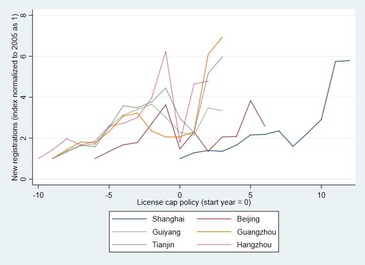
relationship between income and new registrations. Another potentially relevant policy
is the cap that some Chinese cities, such as Beijing and Shanghai, impose on new license
plates (Li, 2018): a household wishing to add a new vehicle must first obtain a license plate
in a lottery or auction. Income should have a smaller effect on new registrations in such
cities, although if a household already owns a car, it can avoid the lottery or auction by
discarding that car and buying a new one. Column 4 shows that income has a smaller
effect for cities with license plate caps than other cities, although the coefficient is small.
Next, we turn to dynamics. In principle, mean reversion in income and new car
registrations could explain the large effect that we estimate. To illustrate this possibility,
consider a hypothetical city that experiences simultaneous negative shocks to income and
new vehicle demand prior to our sample. If both income and new vehicle demand are
mean reverting processes, we would estimate a positive relationship between the two
variables even if the relationship is only spurious. To allow for the possibility of such
mean reversion, we compute quintiles of city income using the 2005 distribution. Column
5 of Table 4 adds to the baseline the interactions of quintile fixed effects with a linear
time trend. These time trends control for potential mean reversion, and adding these
variables would decrease the income coefficient if mean reversion were an important factor.
However, as column 5 shows, adding them causes the coefficient to increase. The estimate
is significant at the one percent level, but the standard error is also larger than in column
1. This reflects the correlations among the instrumented income and the quintile-trend
interactions; the first-stage F-statistic in column 5 is substantially smaller than in column
1. Thus, notwithstanding the large standard errors, we do not find evidence that mean
reversion causes a spurious estimate.
Another issue related to dynamics is the possibility that income has a noncontempora-
neous effect on vehicle demand. That is, the baseline IV specification includes the implicit
assumption that income affects new vehicle demand within a year. In practice, consumers
may delay making a new car purchase after their incomes increase for a variety of reasons,
such as waiting to determine whether the increase is permanent. Ideally, we would test for
such dynamics by adding lags of income to the baseline specification, but unfortunately,
current income is highly correlated with lagged income. Therefore, in Table 5 in columns
2–4, we replace current income with the one-, two-, or three-year lag (column 1 repeats
the baseline). If consumers respond to rising income with a lag, the income coefficient on
lagged income would be larger than on current income, but the table shows that this is
not the case. Therefore, we do not find evidence refuting the hypothesis that new vehicle
purchases respond to income within a year; put differently, if purchases respond with a lag,
21the lagged response is no larger than the estimated contemporaneous response.
Table 5: Effects of Lagged Income on Vehicle Registrations
(1) (2) (3) (4)
Dependent var: log new registrations Current 1-year lag 2-year lag 3-year lag
Log income 2.53 2.85 2.96 2.59
(0.39) (0.42) (0.42) (0.45)
Observations 3,627 3,348 3,069 2,790
Effective F stat for IV 83.33 76.06 67.99 60.59
Kleibergen-Paap stat 44.95 43.62 41.89 39.24
Underidentification p val 0.00 0.00 0.00 0.00
Notes: The table reports coefficient estimates with standard errors in parentheses, clustered by city.
The dependent variable is the log of registrations. All regressions include city and year fixed effects
and province–year interactions. The first column uses current period log income. Columns 2–4 replace
current log income with one-, two-, or three-year lags of log income, instrumented by the corresponding
lag of the instrument.
Estimating equation 3 yields the sample average elasticity of new registrations to
income. As noted, because the income distribution may affect registrations rather than
average income, the elasticity could vary across cities or with income. In Table 6, we allow
the income coefficient to vary across cities according to the city’s 2005 income. Columns 1
and 2 assign each city to one of two groups, depending on whether its 2005 income is below
or above the median 2005 income. Columns 3 and 4 include three equal-sized groups
based on 2005 income. The table shows that the effect of income on new car registrations
is larger for initially high- than low-income cities, but the difference across city groups is
small; columns 1 and 2 show that the high-income city coefficient is about 5–10 percent
higher, and columns 3 and 4 show that the effect is 10–20 percent higher, depending on
the specification and group. However, note that the first-stage F statistics are smaller than
in the baseline, particularly when we consider three groups. This indicates that although
the instrument has sufficient variation to identify the baseline specification, unfortunately,
variation is insufficient to consider much heterogeneity.
22You can also read