The importance of being earners: Modelling the implications of changes to welfare contributions on macroeconomic recovery

Munich Personal RePEc Archive

The importance of being earners:
Modelling the implications of changes to
welfare contributions on macroeconomic
recovery

Mosley, Max

CEPR, LSE

23 June 2021

Online at https://mpra.ub.uni-muenchen.de/108620/
MPRA Paper No. 108620, posted 07 Jul 2021 13:19 UTC

The Importance of Being Earners:
 Modelling the Implications of Changes to
 Welfare Contributions on Macroeconomic
 Recovery.
 Max A. Mosley
 Covid-Economics, Issue 82, pp. 99-142, CEPR Press
 June 23, 2021

 Abstract

This paper demonstrates how changes to welfare generosity during recessions induces a
greater than usual economic response. This is predicated on the assumption that welfare
recipients are likely to be liquidity-constrained and therefore highly responsive to a
change in temporary income. This would result in two conclusions, (i) the effects of fiscal
stimulus can be maximised when channelled through welfare and (ii) fiscal consolidation
from these programs will have a strong contractionary effect on domestic output. Using
tax-benefit microsimulation model UKMOD, we find 71% of means-tested welfare
recipients are liquidity-constrained. We use this finding to calibrate an open-economy
New Keynesian macroeconomic model to therefore illustrate the economic implications
of positive changes to the program’s generosity, finding an impact fiscal multiplier of
1.5. For cuts to contributions, we find a negative multiplier of 1.8, implying past cuts to
welfare had a sizeable contractionary effect on macroeconomic recovery.

JEL: E62, H53, B22, E21

Keywords: Liquidity-Constrains, UKMOD, Fiscal Policy

Acknowledgments:
I am particularly grateful for the guidance, support and engagement Professor Andrés Velasco has given
this work. I would also like to thank Dr Evan Tanner, Dr. Iva Tavessa, Professor Kitty Stewart, Sir Julian
Le-Grand, Charles Morris and Sam Anderson for their individual contributions to the ambitions of this
paper. The results presented here are in part based on UKMOD version A2.50+. UKMOD is maintained,
developed and managed by the Centre for Microsimulation and Policy Analysis (CeMPA) at the
University of Essex. The process of extending and updating UKMOD is financially supported by the
Nuffield Foundation. The results and their interpretation are the author’s responsibility

 -1-

1. Introduction
Following major contractions in output, governments can stimulate economic activity
by purchasing infrastructure or cutting taxes/transferring cash to defined households.
The need for such interventions has been made more necessary while monetary policy –
which has the power to pull back on or even fully offset any expansionary effect of fiscal
stimulus – remains constrained at the zero-lower-bound; this has resulted in fiscal policy
taking a renewed frontline role as a stability mechanism (Shoag, 2013).

The efficacy of cash-transfers – which are often the most appropriate method of
stimulus delivery due to the comparatively short implementation time – is dependent on
recipients choosing to spend the windfall. However, the Barro-Ramsey model in
standard consumption theory predicts that temporary income variations will not induce
a consumption response as households will save any temporary windfall in anticipation
of a future tax rise to pay for it (Barro, 1974). This suggests such households have a
marginal propensity to consume (MPC) of 0. If stimulus is not spent and instead saved in
its entirety, the ratio of the output increase to stimulus, known as the fiscal multiplier,
will be at or close to 0, rendering the intervention ineffective.

This simple model assumes that all households have equal access to alternative sources
of cash (savings) or debt (credit markets) to act as a buffer to any income shock to allow
the household to finance a permanent level of consumption (Canbary & Grant, 2019).
However, a large amount of empirical literature, starting with Hall (1978), has
consistently found 20% of households do not adhere to this permanent income
hypothesis because they have little savings and/or are excluded from credit markets
(hereafter referred to as liquidity-constrained). This inability to draw on alternative
sources of liquidity shortens the horizon for financial planning (Campbell & Hercowitz,
2019), resulting in this subset of households being therefore highly sensitive to a change
in temporary income (Jappelli, et al., 1998; Jappelli & Pistaferri, 2014; Parker, Souleles
and Johnson, 2006; Johnson, et al., 2006). As such, papers that model the fiscal
multiplier only for liquidity-constrained households often find strong responses, with
Kenichi Tamegawa (2012) concluding:

 -2-

“The maximum value of the multiplier is obtained when the share of
 liquidity-constrained households is close to unity” (Tamegawa, 2012)

If liquidity-constrained households are the strongest – and arguably sole – demand-side
channel for stimulus, can governments maximise its multiplier by making it available
only for these defined households? Historic cash-transfers have, to the best of our
knowledge, never been made available to just households with low savings/credit
market access. This is likely for two reasons: firstly, it would take a large administrative
effort to identify households who meet this criterion, involving a lengthy and dangerous
delay while governments audit each household’s total financial assets. Secondly, it would
likely be too politically difficult to justify transferring stimulus to these households
exclusively as to the general population this could appear to be a somewhat arbitrary
criterion for stimulus checks.

Consequently, if the onus for stabilising short-term outcomes has fallen on cash-based
fiscal stimulus, but this can only influence economic activity when liquidity-constrained
households gain, the policy is at best inefficient if we currently have no realistic way to
target them specifically. Many therefore argue fiscal stimulus to be ‘too circumscribed’
(Cochrane, 2010) if it can only influence a small subset of the population. Cochrane’s
challenge to any proponent of fiscal stimulus is that they must either disprove the claim
that the majority of households consume from their permanent income or find a way for
stimulus to better target these liquidity-constrained households.

This paper assesses the role of existing welfare programs in meeting this latter challenge,
as means-tested social assistance, by definition, is only available for households with low
savings. For instance, the United Kingdom’s (UK) Universal Credit scheme’s strict
criteria means that recipients can only claim state assistance if a household’s total
savings are less than £16,000 (DWP, 2021). Therefore, these programs appear naturally
designed to benefit liquidity-constrained households. If this is the case, the following
conclusions would result.

Firstly, fiscal multipliers can be maximised when stimulus is channelled through these
programs as they would present the most effective way to transfer cash directly to the

 -3-

households who are liable to spend it. This presents little administrative challenge, as
raising the levels of existing structures can be enacted quickly; the £20 boost to
Universal Credit was enacted a few weeks following COVID-19 restrictions (HM
Revenue & Customs, 2020). This would also likely be politically feasible, as public
support for raising welfare levels during recessions is usually high, with 74% of the
public being in favour of the aforementioned boost to Universal Credit (Ipsos MORI,
January 2021).

Secondly, fiscal consolidation from cuts to welfare will induce a stronger contraction in
domestic consumption and thus output. The Bank of England provide one of the only
estimates of MPCs from both increase and falls in income; they find consistently higher
estimates from the latter than the former (Bunn, et al., 2017). If liquidity-constrained
households are not only the most responsive to a positive change in temporary income
but are even more responsive to negative shocks, this implies that consolidating welfare
spending would induce a strong contractionary effect on domestic consumption.

This is not the first paper to assess the role of liquidity constraints in strengthening fiscal
multipliers but is, to the best of our best knowledge, one of the first in assessing the role
of welfare programs in achieving this goal. We believe the study of fiscal multipliers out
of welfare programs has only ever been studied once before by Gechert et al (2021) for
Germany, who note a similar dismay at the lack of academic attention given to the
question. They opt for the popular (s)VAR strategy to estimate the multiplier of
exogenous shocks to welfare implementation, finding consistent multipliers of 1.1 as a
result of the strong representation of liquidity-constrained households in the program.
The AARP similarly studied the general question of how welfare is connected to the
domestic economy by using an ‘off-the-shelf’ impact assessment model IMPLAN to
measure this, finding it supported $1.4 trillion in output in one year (Koenig & Myles,
2013). Though compelling, the approach fundamentally lacked any econometric detail,
asking the reader to focus solely on the outcome and forego any consideration for how it
was arrived at.

 -4-

The first contribution this paper seeks to make arises by centring its analysis on the
United Kingdom, where existing welfare generosity ranks low compared to other
European nations. Specifically, the UK’s replacement rate, that is the proportion of
average income replaced by unemployment benefits,1 ranks the lowest on a range of
measures (Spinnewijn, 2020). This is important, as the reader could agree that welfare
programs provide a strong avenue for stimulus but claim that this already happens
following a recession when more people become eligible for welfare, known as an
automatic fiscal stabiliser. But the ability for the UK’s automatic stabiliser to enact the
above is weak if its welfare programs are already meagre, meaning the UK government
cannot rely on its existing programs to stimulate demand without an additional stimulus
boost. As a result, it is common that countries with low automatic stabilisers (such as the
UK) enacting higher levels of stimulus during economic crises (Dolls, et al., 2012) and
vice versa.

Our paper first confirms the fundamental assumption that welfare programs already
target this strong demand side channel by determining how many liquidity-constrained
households benefit from the program compared to tax-cuts as an alternative. We do this
by using tax-benefit microsimulation model UKMOD which can simulate the
distributional consequences from changes to both welfare and tax levels using data from
the 2018 Family Resources Survey (FRS). We simulate the effects of changes to welfare
policies and tax-rates and compare the number of liquidity-constrained households that
gain. As this is a static model, it can only show the ‘morning after’ effects of a policy or
policy reform and cannot initially solve for core macroeconomic outcomes such as the
relationship between the program and demand stimulation. This paper therefore takes a
novel approach to UKMOD, by using it to test core assumptions we can then use to
build an accurate macroeconomic model.

The macroeconomic model we opt for is an open-economy New Keynesian extension of
an IS/LM setting created by Tanner (2017). We use this model to solve for core macro
variables such as the output gap and thus draw inferences about the multiplier effect

1 Spinnewijn measures at the start of an unemployment spell for a representative 35-year-old worker with

an employed partner and one child earning the respective countries average salary before unemployment
spell.

 -5-

from different fiscal policy designs. As this model is simpler and relies on a number of
exogenous parameters, we provide transparent robustness checks that calibrate the
model so that its outputs are consistent with historical outcomes. We assess the size of
the multiplier from positive and negative changes to welfare contributions on core
macroeconomic outcomes, consumption/investment/net exports etc.

Typically, papers of this nature would attempt to estimate effects using either a
quasi/natural statistical experiment or use comprehensive DSGE/(s)VAR models.
Regarding the former, changes to welfare contributions happen at either micro-level
(such as the regional roll-out of a new welfare program) where there is insufficient
micro-data to determine the causal effect from, or the macro-level (country-wide) where
it is not possible to disentangle the effect of the welfare reform from other economic
factors. Papers instead often opt for the latter set of sophisticated economic models
which can estimate comprehensive, dynamic economic outcomes following hypothetical
policy shocks. However, such complex models are naturally computationally intensive,
making them particularly inaccessible to even seasoned economists (Krugman, 2000).
This has brought them into sharp criticism by high profile economists, including
Blanchard (2009) and Romer (2016) for their inability to communicate salient economic
policy to policy makers. These models are therefore better suited in providing
evaluations of economic outcomes for more academic audiences.

The simpler static model employed in this paper can aid more transparent
communication of the key macroeconomic relationships and outcomes to a potentially
non-technical audience. This approach aims for something of a middle-ground between
the two methods above, to test for and demonstrate the intuition of this paper. However,
what we gain in transparency we lose in economic precision, so this paper can be seen
as an illustration of this position regarding the role of welfare programs in fiscal policy.
This gives future papers in this area with more robust models a benchmark to compare
results to.

This paper takes a novel approach to optimising fiscal stimulus, assessing the role of
existing welfare programs by using transparent and intuitive econometric methods. We

 -6-

also extend this position to estimate the contractionary effect of cuts to these programs,
thus providing a comprehensive account for how changes to the generosity of welfare
contributions can influence economic recovery. The paper is organised as follows. A
conceptual framework in section 2 will outline key literature on fiscal stimulus and
liquidity-constraints. Section 3 will outline the methodology for both the
microsimulation technique and the key features of the macroeconomic model. Our
findings will then be split the outputs from the microsimulation and the macroeconomic
model in section 4 and 5. The implications from both sets of findings are considered in
the discussion in section 6.

 2. Conceptual Framework

2.1 Review of Literature and Debates Over Fiscal Policy
How effective fiscal policy is in influencing the economic outcomes has been long
debated by economists. Investigations of historic fiscal multipliers over the post-war
period have taken broadly two forms of inquiry; first, papers that track the observed
economic effects of exogenous build ups of post-war military spending as a natural
experiment; finding multipliers ranging from 0.6-1.6 (Edelberg et al ,1998; Hall, 2009;
Ramey, 2009; Nakamura & Steinsson, 2011). The second kind utilises structural vector
autoregressions (SVAR) to empirically test for past multipliers and its determinants,
finding multipliers from 1-1.5 (Blanchard and Perotti, 2002; Ramey, 2011; Gechert,
2021). More recently, the 2008 US stimulus package was prominently stated to have a
multiplier of 1.6 by the Chair of Council of Economic Advisers to President Obama (as
cited in Ilzetzki, et al., 2013). This drew sharp criticism from Robert Barro, who argued
the output multipliers are near 0 as the gains from government purchases are partially
or fully offset by the negative impacts they have on private investment (Barro, 2009).
Barro later calculated that the extra $600bn in this stimulus spending came at the cost of
$900bn fall in private investment (Barro, 2010), implying a multiplier of just 0.6.

How do we reconcile these competing views? It could be that the economic
environment today is no longer as hospitable to fiscal interventions as it was in the post-
war period. Ilzetki et al (2013) provide evidence for this, by identifying the key
characteristics that determine the size of these historic spending multipliers by

 -7-

employing the same SVAR strategy as Blanchard & Perotti (2002). One notable feature
they find of multipliers is that they are strongest in low-debt (

recession to avoid these implementation lags. For instance, the United Kingdom was
able to enact its furlough program in 2020 three days before lockdown even began.

The efficacy of cash-transfers will depend on the amount of the temporary transfer that
is spent by households, measured by the marginal propensity to consume (MPC).
Economists have long been sceptical that households would ever spend a temporary
gain (implying an MPC of 0), as the majority of households will only consume out of
their permanent, as opposed to temporary, income and therefore save the entirety of the
windfall in anticipation of future tax rises to pay for the stimulus (Barro, 1974;
Cochrane, 2010). Although this has been found to apply to well over the majority of
households (Hall & Mishkin, 1982; Canbary & Grant, 2019), households with low-
savings and little access to credit markets are in fact highly responsive to both positive
and negative temporary income changes (Johnson, et al., 2006). For these households,
studies have estimated MPCs as high as 0.92 (Canbary & Grant, 2019) as they cannot
smooth consumption out over the life course.

2.2 Defining Liquidity Constraints
There is some variation in how previous studies have formally defined a liquidity-
constrained household, given the fact ‘low savings’ is an ambiguous term. There are
four compelling sets of criteria that attempt to isolate households from sources of
plausible earnings: (i) savings, (ii) market earnings, (iii) home-owners or (iv) credit
markets. The first is captured by the Zeldes definition, which classifies liquidity
constraints as households with total wealth of less than two months disposable income.
Although this neatly captures a lack of savings relative to a household’s given earnings,
measurement of household wealth is often prone to error and datasets often do not
collect it for this reason (Jappelli, et al., 1998). Further, this definition only works if the
relationship between wealth and liquidity constraints is perfectly monotonic (Dolls, et
al., 2012).

Runkle (1991) therefore focuses on the second and third sources by considering all
unemployed households without a mortgage as liquidity-constrained. The clear logic

2 Meaning for these households, 90% of the income gain will be spent in the domestic economy

 -9-

behind this approach is that unemployed households (where there is no adult working)
with no income and no ability to liquify the capital stored up in their home will have
little opportunity to smooth out the temporary income shock. The fourth is perhaps the
most difficult to obtain data for, as credit market statistics will be held only by private
stakeholders. It is therefore common to use survey data that directly asks households
about their access to credit, as Jappelli et al (1998) and Dolls et al (2012) do, such as with
the FCA financial lives survey which asks participants if they have had a rejected credit
application (FCA, 11 February 2021, p. 123).

Due to data and methodological constraints explained below, we opt for a combination
of the second and third measure. As we will be using tax-benefit model UKMOD to
determine which forms of fiscal stimulus target liquidity-constrained households the
most, we are therefore limited by the variables available in Financial Resources Survey
(FRS) dataset the model relies on, meaning we cannot at this stage use the FCA dataset.
Unfortunately, there is little data on savings/wealth, meaning we cannot take the first
approach in its entirety. Instead, we build off the second approach, identifying all
households who do not own their own home and with no working adults3 to be
liquidity-constrained. Lastly, we include a fifth source of income; (v) the household
having no investment income.

2.3 The MPC for Liquidity-constrained Households
Many papers that attempt to identify MPCs for households from transitionary gains
often differentiate between representative and liquidity-constrained households for this
reason, as the consumption response for a household with low savings and without
credit market access will be higher than the population. A summary of this literature is
presented in Table 1, which shows that MPCs are consistently found to be higher for
liquidity-constrained households than typical households under range of scenarios and
country-settings. For each study, we see far higher MPCs when looking at just liquidity-
constrained households than at the overall population.

3 We drop this unemployment requirement when looking at tax-cuts, explained below

 - 10 -

Table 1: Literature Estimates of MPCs
 MPC Estimates
 Liquidity-
 Author(s) Context/Sample Overall Notes
 constrained
 2011 Growth Estimate is at both
 Agarwal and Qian
 dividend 0.8 0.5-0.75 announcement &
 (2014)
 (Singapore) dismemberment
 First of many
 papers that uses
 Johnson, Parker 2001 US Income
 0.2-0.4 Larger random timing of
 and Souleles (2006) Tax Rebates
 stimulus-based
 welfare number
 Johnson, Parker 2008 US
 Same method as
 Souleles and Stimulus 0.5-0.9 Larger
 above
 McClelland (2013) Payment
 Tullio Jappelli & Low ‘cash-on-hand’
 2010 Italian
 Luigi Pistaferri 0.48 0.7 households exhibit
 Dataset
 (2014) larger MPCs
 0.75-0.94 Find only 50% of
 Zara Canbary and
 1986-2010 UK (higher households
 Charles Grant 0.5-0.94
 FRS Dataset following consume from
 (2019)
 recessions) permanent income
 MPC tapers off to 0
 1999-2013 US
 Fisher et al (2019) 0.2-0.6 Larger after the 3rd wealth
 PSID Dataset
 quintile
 0.37 Measure effects of
 Tal Gross, Matthew US Consumer
 (20-30% higher bankruptcy flag
 Notowidigdo, and Credit Panel -
 during great removal on
 Jialan Wang. (2016) (CCP)
 recession) consumption
 Do not test for
 liquidity-
 Survey over
 Crossley et al (2021) 0.11 - constrained
 COVID-19
 households
 specifically

Despite the fact these estimates are found from variance in study type, each consistently
shows that the MPC is highest for liquidity-constrained consumers. This is likely because
the basic intuition is the same, households with low access to alternative sources of cash
will be responsive to temporary income changes. For our analysis, we take Canbary and
Grant’s estimates as true representations of the MPC for liquidity-constrained
households as their estimates are for the UK (thus eliminating the effects of any country
specific factors) and is estimated from the dataset we use in UKMOD. We then apply
this MPC to the percentage of liquidity-constrained households within welfare programs
identified in our microsimulation exercise. For these liquidity-constrained households

 - 11 -

we can assume with some certainty a change in temporary income will induce a strong
change in consumption as they do not have alternative income sources to draw on.

Existing literature has identified the need for cash-based fiscal stimulus and specified the
households it needs to target, but there is a gap in understanding how best to achieve
this. Therefore, this paper explores the role of welfare policies in meeting this challenge
and will evaluate if existing programs already benefit liquidity-constrained households.
If so, we will be able to illustrate the economic consequences of positive and negative
changes to welfare using a macroeconomic model.

 3. Methodology

For studies of this nature, there are two possible methodological candidates. The first is
to test for economic outcomes following real-world changes in welfare contributions by
determining their causal effect using quasi/natural experiments. However, this has not
been possible due to data constraints, as the changes we can track are on a micro scale
whereas the available data on economic indicators (such as consumption levels) are
aggregated. Further, this approach does not give us a plausible avenue to explain why
we observe a given outcome. This paper is based off existing economic intuition about
the role of liquidity-constrained households in strengthening the effects of fiscal stimulus,
but quasi/natural experiments do not give us the opportunity to determine if it is this
that is driving our results or if it is being driven by some other factor.

Instead, studies of this sort opt for the alternative class of methodologies is through the
use of sophisticated economic models such as with a DSGE of (s)VAR framework.
Though powerful, these computationally intensive methods struggle to communicate
results to a non-statistical audience (Krugman, 2000) and have therefore been criticised
for their lack transparency (Romer, 2016).

Our methodological approach has been chosen as something of a middle-ground
between these two approaches, that is built off real-world observations and estimates
results using a less intensive New Keynesian extension of an IS/LM macroeconomic
model. Therefore, our methodology is split into two approaches. The paper first tests for

 - 12 -

the fundamental assumption that welfare programs target liquidity-constrained
households through the use of microsimulation model UKMOD. We then estimate the
fiscal multiplier effects of a hypothetical change in the levels of contributions using this
macroeconomic model.

3.1 Microsimulation through UKMOD
We first confirm the fundamental assumption that existing welfare programs target
liquidity-constrained households using the tax-benefit microsimulation model
UKMOD. This model is built from the 2018 Financial Resources Survey (FRS) which
provides figures on the personal and financial characteristics of the population, and
welfare recipients specifically. This official dataset provided by the Office for National
Statistics (ONS) is a continuous survey of UK households, comparable to EU-SLIC,
which provides statistics on income sources and general characteristics including home
ownership.

The UKMOD microsimulation model opens up opportunities to simulate tax-benefit
changes and assess the distributional consequences. Specifically, we can simulate an
increase in benefit levels and determine what proportion of those who gain are liquidity-
constrained. We therefore code 1 for those who see an income change and 0 otherwise.
We apply this analysis to each type of UK benefit to determine the presence of any
heterogeneity across programs. It is likely that means-tested benefits are better able to
target liquidity-constrained households than non-means tested benefits, as the former is
designed to specifically target financially precarious households whereas the eligibility
for the latter is not necessarily savings/credit related (e.g., child benefit). This UKMOD
model focuses analysis on taxes and benefits applied to the whole of the UK and
assumes full benefit take-up and tax-compliance at the household unit level. As this is a
controlled microsimulation experiment, we do not have to worry about endogeneity
issues, as we are able to isolate the effects of the given changes to taxes and/or benefits.
Improvements to this approach are specified in section 6, specifically how new datasets
can be added and more analysis across different time periods would improve the overall
precision of our estimates and their generalisability.

 - 13 -

We can compare these results to cuts in tax-rates to see how many liquidity-constrained
household’s gain. As it is common for stimulus through tax-cuts to be targeted at ‘lower’
income households, such as the 2001 US tax-rebate (Johnson, et al., 2006), we therefore
simulate this tax-cut on the lowest those tax-bands; again coding 1 for those who see an
income change and 0 otherwise. As mentioned above, there are a number of ways to
define ‘liquidity-constrained’ households and we include ‘unemployment’ as a key
feature. However, for tax cuts this would result in no liquidity-constrained households
gaining as they would not be earning market income under this strict definition.
Therefore, for the tax-cut stimulus simulation we drop the unemployment criteria
(keeping the no investment and/or non-homeowner measure).

This can provide a robust account of how different designs of stimulus can target more
or less liquidity-constrained households which is presented below. This can therefore
help us identify what is the appropriate average MPC for welfare recipients or those
who benefit from a tax-cut.

3.2 Constructing a Macroeconomic Model
If welfare programs do target liquidity-constrained households, we can illustrate the
implications of stimulus through these strong demand-side welfare programs by
calibrating a macroeconomic model. The model we use is detailed in Appendix A and
specified in full in Tanner (2017), but here we outline how the IS curve, interest rates
and output gap are calculated. This allows us to produce multiplier estimates of fiscal
shocks measured as a percentage of potential output. First, we substitute the rescaled
equations in Appendix A for consumption, investments and net exports into a New
Keynesian GDP identity, including a measure for government purchases ! :

 ! = " ∗ [1 + )1 − #$# ,{[(1 − )( ! )] − ! } + %& ( ! − r) + ! ]

 %& is a response parameter scaled to potential output, so that %& = & / " . We then
subtract and divide both sides by potential output to solve for the output gap IS curve:

 - 14 -

 %& ( ! − r) + ! − )1 − #$# , !
 ! =
 σ

comparing the percentage change from period 1 to period 2 (the latter with the policy
shock). We input this into a demand shock component which eventually interacts with
the MPC )1 − #$# ,. This builds this intuition that MPC size is what leverages the size
of the economic response. The inclusion of the MPC estimate allows us to model effects
of any scenario based on its distributional effects to different households. This can show
the implications for fiscal policy to both Ricardian equivalence/permanent income
households with an MPC of 0 or liquidity-constrained households with an MPC>0
defined using Table 1. Further, this model can show how fiscal policy can appreciate or
depreciate the real exchange rate depending on the relative strength of the monetary
response in a more transparent and intuitive way than complex DSGE methods. This is
of key importance for this paper, as it can show in a credible way how different
monetary conditions (ZLB) can strongly influence the effectiveness of fiscal policy.

We can therefore compare the effects of the expansion in a number of scenarios which
are (i) during a minor recession where monetary policy has room to respond to both the
recession and expansion, (ii) during a major recession at the zero-lower-bound with a
capital outflow scenario. We then replicate this latter analysis by decreasing welfare
contributions.

Of course, this model does have a number of notable constraints that limit what can and
cannot be inferred from its estimates. Firstly, this is only a static model in the same form
as UKMOD, meaning we cannot forecast into the future what the outcome will be after
multiple rounds of spending. Many papers that estimate fiscal multipliers do this (see
Blanchard & Perotti, 2002; Ilzetki et al, 2013) to see how long it takes for the effect to
equalise; we are unable to make such analysis from this model. Secondly, such New
Keynesian models have multiple exogenous variables which are independent from the
policy change. Notably, our nominal exchange rate ! (see Appendix A) is exogenously
defined, meaning it is not connected to the given economic conditions so an
appreciation in the current account following stimulus will not result in capital inflows.
We therefore incorporate this with a forcing variable by decreasing external financial
pressure by 0.1% to induce a capital inflow scenario, consistent with the set-up Tanner
(2017) performs. For simplicity we assume this inflow is linear across MPC estimates,

 - 16 -

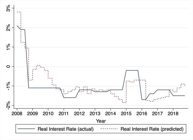
when in reality it will be dependent on the output response. Although this may help us
avoid overestimating some results, the approach is imprecise in nature and is less
convincing than a model that is able to do this naturally.

The ‘Lucas Critique’ refers in part to this problem of believing elements of structural
equations to be exogenous, as even aspects of consumption are never truly independent
from government policy (Sargent, 1987). As such papers opt for the more sophisticated
models of SVAR and DSGE models mentioned earlier which are far better able to
overcome these limitations.

Therefore, this model should be taken as an economic illustration of the above
argument rather than a direct forecast for the UK. It would be a worthwhile exercise to
cross-check this model with one of these other approaches, as Pappa et al (2015) do
when assessing the impact of tax avoidance on fiscal consolidation. Such further
research opportunities are addressed in section 6.

3.3 Robustness Checks
Because of these fundamental limitations in the precision and interpretability of our
model, we believe it necessary to disclose its relative power by cross-checking its outputs
from historical events to what they were in reality. We do this on the key variables that
exert the strongest influence over our model, real and nominal interest rates along with
inflation shown in Figure 1. We take historical data on output gaps calculated by the
Office for Budget Responsibility (OBR, 2020) and past estimations of the natural rate of
interest by Goldby et al (2015) and input this into the model to allow it to forecast what
the outcomes would have been in the past and compare them to reality.

This exercise can also be helpful in choosing the values of certain exogenous
parameters, such as those that make up the central bank’s Taylor Rule or fundamental
features of an economy such as the elasticity of short run aggregate supply. We therefore
choose a number of parameters to minimise the distance between historic outputs and
the predictions of our model. In doing so we obtain the following parameters in Table 2,
taken either from existing papers or calibrated ourselves.

 - 17 -

Table 2: List of Exogenous Parameters
 Parameter Description Source Value
 ! Inflation expectation Assumption 0.02
 # Inflation target Assumption 0.02
 $ Inflation weight Author’s calibration 2
 %&' Output gap weight Author’s calibration 1
 (( Supply-shock weight Author’s calibration 1
 )*+) Short run elasticity of aggregate supply Author’s calibration 2
 ,+- Natural rate of interest4 Evans (2020) 0.015
 ./. Short-run propensity to import Author’s calculation5 0.126
 # Tax policy (one-off) Policy shock -0.01
 01(. Deviation from Taylor-Rule6 Assumption 0
 ! External financial pressures Assumption -0.01
 Transmission of external shock to Tanner (2017)
 0.10
 exchange rate
 ./. Marginal propensity to consume (MPC) Canbary and Grant (2019) 0.857
 Importance of imports Tanner (2017) 0.03
 2 Response function to export prices Tanner (2017) 0.72
 13 Response function to import prices Tanner (2017) -0.72
 Tax share8 IFS (2019) 0.25

For nominal interest rates in Figure 1 panel a, we are able to track pre and post zero-
lower-bound levels well. Our model naturally ‘recommends’ highly negative interest
rates, as it does not consider zero to being a limiting factor like a central bank will
would. As such, in our future estimates below we set up the model to stop itself at 0 if
the output from interest rate policy is negative to avoid creating highly negative interest
rates.

If we simply subtract inflation from this predicted output (0 if negative), we obtain the
following measure of ‘real interest rates’ in panel b, which if we compare to the same
from actual outputs (real inflation subtracted from nominal rates) we see a high degree
of similarity. We could compare this to actual real interest figures, such as those done by

4 For robustness checks we use yearly estimates rather than this long-run value
5 See Appendix B
6 Although we consider this 0, we use this for force adjustments where necessary to keep interest rates ≥0
7 Calibrated as an average of their estimate range for liquidity-constrained households
8 Calibrated to reflect low-income households

 - 18 -

the World Bank, however their inflation deflators are not the same as ours so the
outputs would not be interpretable.

We simulate the effect of the 2015/16 oil shock by imputing a supply shock ( ) of 1%,
as this episode had a substantial effect on inflation (Bank of England, 2016). As such,
although our inflation in panel c is able to track real inflation fairly well, supply shocks
must be simulated manually as the model cannot predict this itself otherwise it would
have not noticed the 2015/16 oil price shock as this would not have been that well
reflected in the output gap.

Figure 1: Robustness Checks

(a) Nominal Interest Rate (b) Real Interest Rate

(c) Inflation

Overall, although our model is constrained in a number of areas, it is able to match
historic outputs fairly well, at times with some adjustments. We are confident that this
gives us a credible basis to illustrate the effects of exogenous changes to fiscal policy
through welfare.

 - 19 -

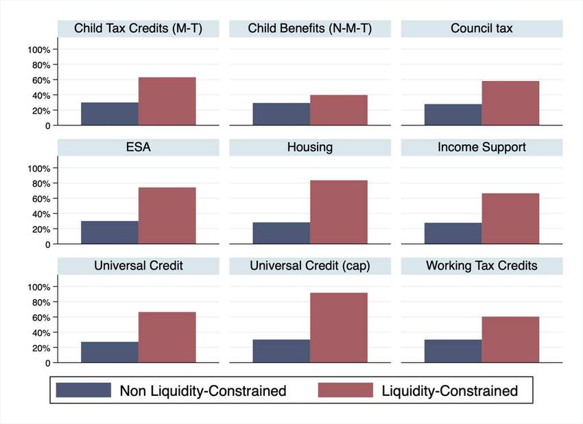
4. Findings: Microsimulation

The microsimulation exercise using UKMOD allowed us to first estimate that 30% of
all households are liquidity-constrained using the criteria mentioned in Section 2, which
is similar to Hall’s (1978) 20% estimate. This at first confirms the concern that fiscal
stimulus targeted at the broad population will be inefficient at targeting liquidity-
constrained households.

4.1 Liquidity-constrained households by benefit category
When we simulate the effects of a change in welfare contributions, we see the following
distributional consequences for liquidity-constrained households9. From broad welfare
programs, we find in total 58.4% recipients are liquidity-constrained. But when we start
to look within the different welfare programs that make up this finding in Figure 2, there
is some important variations. First is the difference between means-tested and non-
means-tested programs.

We take the difference between child tax credits and child benefits as an example of this,
as both are similar in design but only the former is means-tested. For the non-means-
tested program, only 39% of recipients can be classified as liquidity-constrained
compared to 63% of recipients from the means-tested equivalent. This is consistent with
the intuition of this paper that the reason welfare programs can target liquidity-
constrained households is because the criteria to be eligible for means-tested welfare is
very similar to what we would consider a household to be liquidity-constrained (e.g.,
having low levels of savings). When we look at the rest of the means-tested programs, we
see a consistently high proportion of recipients being liquidity-constrained. Notably, we
can infer that 91% of households impacted by the Universal Credit cap are liquidity-
constrained. Overall, we find 71% of means-tested welfare recipients are liquidity-
constrained, but just 27% are in non-means-tested programs; similar to the wider
population. This intuitive, as without strict eligibility criterions in non-means-tested
programs the demographic make-up of recipients will more broadly reflect the
population.

9 These are the same for both positive and negative changes to contributions

 - 20 -

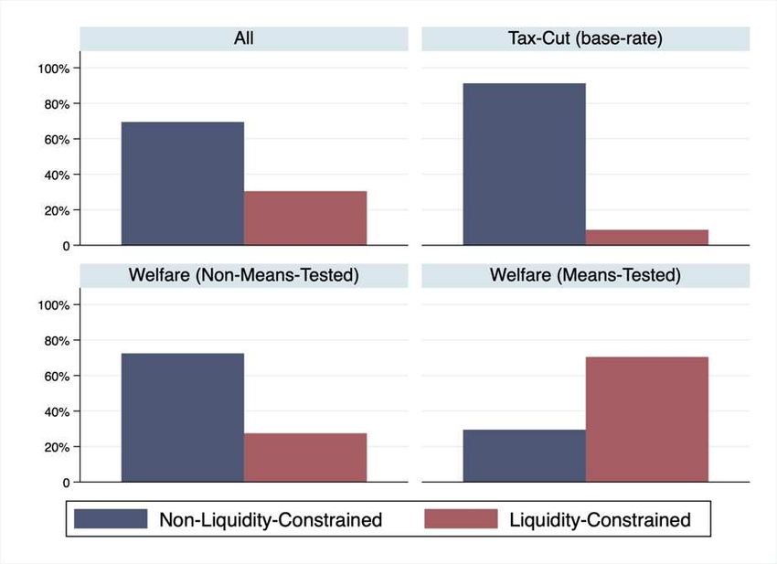
4.2 Liquidity-constrained households by Tax Cut
We then repeat this exercise by simulating the effects of a tax-cut to lower-income
households to provide some contextual clarity to the above finding. Specifically, we are
interested in determining if the above implication is limited to just welfare programs, or
if tax-cuts also have this ability to benefit liquidity-constrained households.

 Figure 2: Liquidity-Constrained Recipients by Welfare
 Program

 Source: Authors Calculation through UKMOD

We use UKMOD to simulate a tax-cut through from a 1% reduction in the liability
within lowest basic-rate (£12,571-£50,270) tax band. We again code households who
see a rise in disposable income 1 and solve for liquidity-constrained and non-liquidity-
constrained households. We only simulate a tax-cut for the bottom band to make for a
plausible comparison for stimulus through welfare programs. Our analysis in Figure 3
shows tax-cuts, even on the lowest income band, are particularly inefficient in benefiting
liquidity-constrained households especially when compared to welfare programs; this is
despite dropping unemployment from the definition of liquidity-constrained households
for this analysis. We find 8.7% of households who benefited from tax-cuts through the
base-rate are liquidity-constrained; this reflects the fact that although liquidity-

 - 21 -

constraints will likely correlate with income (low savings households will likely have low
incomes) they do not do so perfectly.

 Figure 3: Liquidity-Constrained Recipients by Welfare
 and Tax Bands

 Source: Authors Calculation through UKMOD

These findings prove the difficulty in designing fiscal stimulus to target liquidity-
constrained households due the fact they only make up 30% of the population. Even
tax-cuts to low-income households are imprecise in nature in achieving this aim.
Instead, we can conclude from these findings that welfare programs present the most
effective way to target these households as a result of their means-tested eligibility
criteria closely matching what we would consider liquidity-constraints. Further, the
reverse is also true, that fiscal consolidation by tax rises will not target as many liquidity-
constrained households as cuts in welfare contributions will. The implications of these
findings are discussed in section 6.

 - 22 -

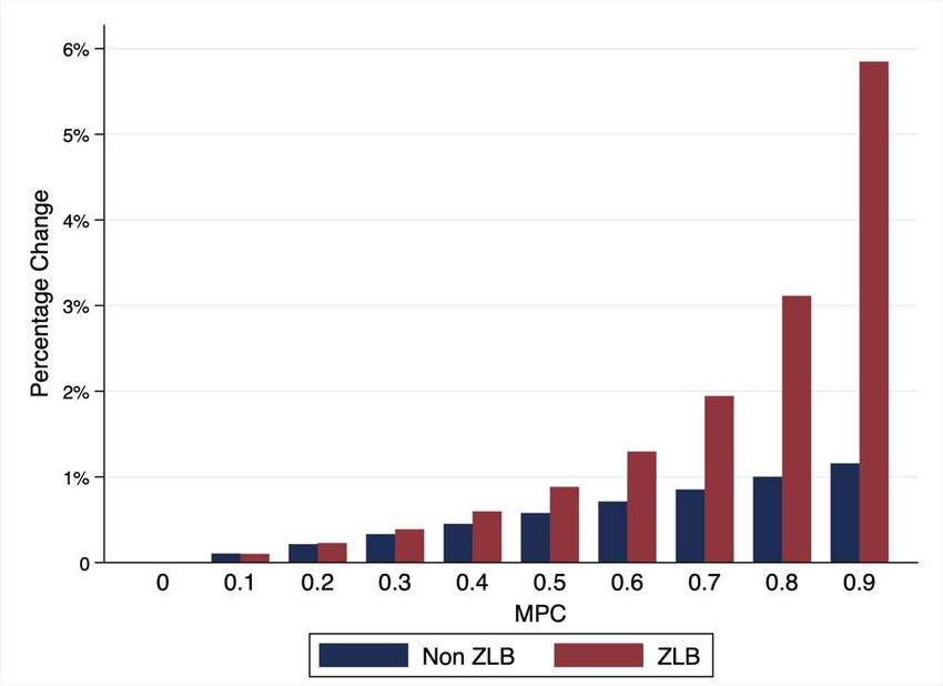
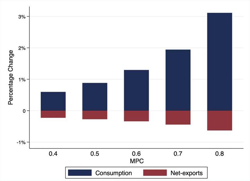
5. Findings: Macroeconomic Model
Now that we have established that fiscal policy through welfare programs can target
liquidity-constrained households, we can use our macro model to illustrate why this will
strengthen the effect of fiscal stimulus and consolidation. Our model does not have the
capacity to consider the implications for how the stimulus is financed on our estimates.
Therefore, we could assume in all instances that stimulus is money-financed by
‘helicopter-drops’ by the central-bank, as such financing arrangements have little to no
effect on multipliers and are similar to debt-financed10 stimulus in a zero-lower-bound
environment (Galí, 2019).

5.1 Scenario 1: Positive changes to welfare contributions
 5.1.1 After a 3% drop in consumption (non-ZLB)
We begin by estimating fiscal multipliers from expansions in social security
contributions during ‘normal times’ recessions, meaning central banks have the capacity
and mandate to respond to any expansionary effects. This is simulated by a 3% fall in
baseline consumption. Figure 4 shows the effects of expansionary efforts from each
MPC size, with higher MPCs naturally influencing a stronger increase consumption and
decrease in net-exports. This displays why the Barro-Ramsey consumption has such
strong implications for the efficacy of fiscal stimulus, as an MPC of 0, as displayed,
would induce no economic response.

Both relationships are linear, which reflects the central bank’s ability to control the
expansionary effects and avoid exponential increases under a pre-determined schedule.
Under this scenario, the base-rate rises from 0.4 to 0.6 as the MPC rises. Looking at just
consumption, the break-even point of 1 (where governments induce more consumption
than they put in) comes once all beneficiaries spend more than 80% of their stimulus.
But the multiplier effect is positive, meaning that although the central bank controls the
strength of the response, it does not fully offset it as the Taylor Rule construction only
recommends small incremental increases according to its policy rules.

10 See Max Corden (2010) for further detail on the long-run effects debt-financed stimulus

 - 23 -

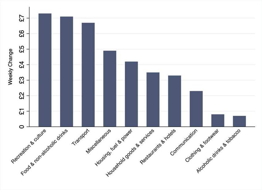
Figure 4: Increase in Welfare Contributions on Consumption
 and Net-Exports by MPC Size (Scenario 1.1)

 Source: Authors Calculation

Consistent with standard Keynesian theory, the effectiveness of expansionary effects is
constrained through the presence of leakages from savings (1-MPC) and imports.
Regarding the latter, if households spend their windfall on imported goods the gain will
not be spent in the domestic economy. Although we are not aware of existing estimates
of the percentage of household expenditure spent on imports, we calculate this ourselves
by multiplying the household expenditure on each commodity by the import
penetration of the given commodity,11 finding 12% of household spending involves
imported goods. We perform this for each household income group and find,
surprisingly, no significant variation when we compare across income deciles as we
would expect when looking at the expenditure of specific commodities (negative
correlation between food expenditure and income). As the expansionary effects
naturally result in a partial strengthening of economic conditions, we see imports
become cheaper and the reverse for exports, resulting in a net loss.

11 See Appendix B

 - 24 -

5.1.2 After a 5% drop in consumption (ZLB)
Scenario 1.2 looks at the above conditions but now increasing the size of recession to a
5% drop in baseline consumption to constrain interest rates at the zero-lower-bound.
This is displayed in Figure 5 where we start to see a more exponential rise in output
following the expansion. Many economic models suggest higher multipliers from fiscal
expansions under this scenario, notably Hall (2009). We find similarly that under this
scenario, not only is the consumption response greater (including a shallower fall in net
exports), but the marginal increase in the multiplier is also positive as the MPC rises.
This reflects the effect of idle monetary policy following an expansion from fiscal
stimulus. We now focus just on the MPCs of 0.4-0.8 as these are the plausible MPC
range of liquidity-constrained households. In doing so we see most of the ‘heavy lifting’
in terms of output increases is being done by the strong consumption response, hence
why the size of the MPC is important in leveraging this output reaction.

As mentioned above, we induce a capital inflow scenario by decreasing external
financial pressures. This results in a higher import response, depressing net exports and
the multiplier. This finding is consistent with other papers that induce capital outflows in
workhorse macro models, such as Blanchard et al (2015) who find short-run
contractionary effects from capital inflows through a reduction in net exports from

 Figure 5: Increase in Welfare Contributions on Consumption
 and Net-Exports by MPC Size During ZLB (Scenario 1.2)

 Source: Authors Calculation

 - 25 -

currency appreciation. The small response in net-exports reflects the central banks
inability to defend the exchange rate, resulting in a smaller fall in net-exports.

The scenarios presented are all under demand-push recessions, meaning the recession is
caused by some shock to aggregate demand (in our case consumption). Of course, this is
not the only form a recession can take. A ‘cost-push’ recession caused, for example, by a
shock to the production process (such as a rise in oil prices) which increases inflation and
causes a contraction in output is conceivable. This situation is often described as an
impossible scenario for policy makers as measures – such as stimulus through welfare
programs – can recover some of the output lost but at the cost of further increased
inflation. When we simulate this potential scenario, we find no response in our output
estimates – as one would expect – but although a supply shock does decrease output and
increase inflation, the fiscal intervention has little further increase in inflation under this
scenario than it does when there is no supply shock. Instead, we find inflation is far
more sensitive to increases when inflation expectations are above the central bank
target. Under both normal times and a zero-lower-bound scenario, any increase in
inflation expectation translates one-for-one into inflation increases. Therefore, the
starting position of inflation is important for policy makers to consider, as our results
suggest the 1% intervention increases inflation by 0.8%, but inflation from stimulus
often takes time to materialise due to price ‘stickiness’ (Galí, 2019). Therefore, it is
important for the policy maker to consider existing inflation levels and a measure of
future expectations. Policy makers must, as always, be cognisant of the fact that
expansions can cause inflationary pressures, which during a zero-lower-bound scenario
can be particularly strong.

 - 26 -

We can show with this model the implications of transferring stimulus to this strong-
demand side channel and show how the presence of zero-lower-bound interest
strengthens the effect of the stimulus boost. Figure 6 compares just consumption
responses under Scenario 1.1 under a normal interest setting and Scenario 1.2 which
zero-lower-bound interest rates. We can see this exponential rise clearly here under the
latter, reflecting the highly responsive economic environment created without the
presence of a monetary response.

 Figure 6: Increase in Welfare Contributions on Consumption
 by MPC Size

 Source: Authors Calculation

5.2 Scenario 2: Negative changes to welfare contributions
 5.2.1 After a 5% drop in consumption (ZLB)
This second scenario assess the impacts from a fall in contributions for these liquidity-
constrained households. This is in part motivated by the finding that households,
especially with low savings, are more responsive to negative income shocks than positive
(Bunn, et al., 2017). This decision was taken by the UK through a number of welfare
reforms between 2013-16, notably through the introduction of a ceiling on the amount
of welfare a household could receive, known as the ‘benefit cap’.

 - 27 -

We therefore take the above setting of a major contraction in output under a zero-
lower-bound scenario, but now reverse the sign of the policy shock to test for the effects
from cuts to welfare contributions. We also reverse the external financial pressure
parameter to induce a small capital outflow response to the depreciation of the current
account that follows, consistent with Tanner (2017).

Our results show, just as scenario 1.2 finds, an exponential effect during the presence of
zero-lower-bound interest rates. Overall, we find the same results as in 1.2 but now with
the sign reversed, resulting in a strong fall in consumption as the MPC rises and a
shallow increase in net-exports due to capital outflows. Figures 5 and 6 can therefore be
flipped to show the effects of cuts to contributions on different MPC sizes.

5.3 Summary
So far, we have shown the response for each MPC assumption. For the summary we
make a decision about the average MPC of all those who benefit from stimulus through
welfare or through tax-cuts based on the above microsimulation exercise. We found a
strong presence of liquidity-constrained households within existing welfare programs,
particularly means-tested, from our microsimulation exercise; therefore, it is appropriate
to consider a high proportion of welfare recipients as obtaining the high MPC range
specified by Canbary and Grant (2019). However, not all welfare recipients are
liquidity-constrained, therefore we assume that the remaining 29% have an MPC of 0,
which will lower the average MPC of all welfare recipients. We take an average from
Canbary and Grant’s range of 0.85 and apply it to 71% of households who benefit and
assume 0 for the rest12, resulting in average MPC of 0.59 out of positive income shocks.
This can be strengthened if the policy maker directs stimulus through specific welfare
programs such as housing benefit which impact’s 84% of liquidity-constrained
households, but for our estimates we take the average across all means-tested programs.
We further apply this analysis to stimulus through tax-cuts to provide a valid
comparison. We found only 8.7% of beneficiaries from cuts to the lowest ‘personal
allowance’ tax band would be liquidity-constrained. Applying the same rules above

12 This is a strict interpretation of the Barro-Ramsey consumption model which may understate results,

but we believe there is merit in providing conservative estimates

 - 28 -

results in an average MPC of 0.8 from tax-cuts to this tax-band; we should note that this
is a lower estimate than the estimates of average MPC from the US tax cut of 0.20-0.40
(Johnson, et al., 2006).

For cuts to contributions, we take use Bunn et al’s (2017) MPC estimate for households
with low net liquid assets to income ratio of around 0.9, which somewhat resembles the
Zeldes definition of liquidity-constraints. Again, we apply this to 71% of means-tested
welfare recipients and assume 0 otherwise, yielding an average MPC of 0.63 out of
negative income shocks. Using these estimates, we simulate the effects of positive and
negative changes to welfare contributions in scenario 1.2 (zero-lower-bound interest
rates) and compare them to stimulus through tax-cuts, obtaining the following results
presented in Table 2.

 Table 2: Multiplier Estimates from Tax-Cuts and Changes in Welfare Contributions
 Tax-Changes Welfare Changes
 Stimulus Stimulus Consolidation

 MPC 0.08 0.59 0.63

 Consumption 0.16 1.25 -1.46

 Investment 0.04 0.59 -0.70

 Net-exports -0.16 -0.33 0.36

 Multiplier 0.05 1.51 -1.79

We now further solve for investment which yields some interesting results. A standard
IS/LM framework suggests investment is directly proportional to savings, so we would
expect as the less is saved and more consumed (as the MPC rises) investments should fall
as Barro (2009) argues. Our results suggest the opposite, that stimulus has a positive
effect on investment and is rising with the MPC. This has been observed in reality,
where the US stimulus checks improved firm level investment due to the increased
profitability at the firm level following the higher economic activity (Correa-Caro, et al.,
2018). Our investment equation summarises the effect of stimulus on investment into
two countervailing forces: the reduction in savings increasing the real interest rate

 - 29 -

reducing investment and the improved output gap increasing it. Our New Keynesian
model therefore suggests the latter force is stronger than the former, likely as a result of
the zero-lower-bound environment.

Overall, our show a strong multiplier effect from positive increases particularly as a
result of the positive effect on consumption, yielding a positive impact multiplier of 1.51.
When we compare this to tax-cuts we see a far lower estimate, with very little impact on
the economy as a result of the far lower average MPC from beneficiaries. For cuts to
contributions, we find a negative multiplier of 1.79 again as a result of the substantial
contractionary effect on domestic consumption as a result of the higher MPC from
negative income shocks. Our results are clearly sensitive to the size of the MPC, as in
our model there is little difference between the positive and negative MPCs from welfare
changes, but we see noticeably different outcomes. This reflects the exponential nature
of Figure 6, which after an MPC of 0.5 grows rapidly. This gives further weight to the
necessity of comparing this paper’s results with estimates from models with greater
precision.

 6. Discussion
Our results have confirmed the key intuition of this paper, that welfare programs target
liquidity-constrained households and subsequent changes to the contributions level of
means-tested programs will has a strong effect on economic outcomes. Our model
suggests every 1-unit increase in means-tested welfare will result in an increase output by
1.5 by improving both consumption and investment, whereas every 1-unit cut will result
in a 1.8 fall in output. This results in two clear policy implications: the economic effects
of stimulus can be maximised when directed through welfare programs, whereas fiscal
consolidation from these programs will have a strong negative effect on output.

It is obvious that these results run contrary to past policy decisions by the UK
government. Specifically, over the course of 2010-15 we saw a strategy of tax cuts to the
top marginal rate and cuts in welfare contributions notably with the introduction of a
‘benefit cap’ in 2013. The latter was justified on the grounds of debt consolidation, with
the stated aim to:

 - 30 -