THE "LIC DETECTOR TOY" PROGRAM
←
→
Page content transcription
If your browser does not render page correctly, please read the page content below
The “LiC Detector Toy” program
                   M Regler, W Mitaroff, M Valentan, R Frühwirth and R Höfler
                   Austrian Academy of Sciences, Institute of High Energy Physics, A-1050 Vienna, Austria, EU
                   E-mail: regler@hephy.oeaw.ac.at

                   Abstract. LiC is a simple but powerful and flexible software tool, written in MatLab, for
                   basic detector design studies (geometries, material budgets) by determining the resolution of
                   reconstructed track parameters. It is based on a helix track model including multiple scattering,
                   and consists of a simplified simulation of the detector followed by track reconstruction using
                   the Kalman filter. After a short description of LiC’s main characteristics, we demonstrate its
                   capabilities by applying this tool in a performance study of the LDC and SiD detector concepts
                   at the International Linear Collider (ILC).

1. The Monte Carlo tool
A simple but powerful and flexible software tool (LiC Detector Toy1 ) for detector design,
modification and upgrade studies has been developed. It aims at investigating the resolution of
reconstructed track parameters in the vertex region for the purpose of comparing and optimizing
the track-sensitive devices and the material budgets of various detector set-ups. This is achieved
by a simplified simulation of the set-up yielding the measured coordinates, followed by full single
track reconstruction.
   The detector model corresponds to a collider experiment with a solenoid magnet, and is
rotationally symmetric w.r.t. the beam axis; the surfaces are either cylinders (barrel region)
or planes (forward and backward regions). The magnetic field is homogeneous and parallel to
the beam axis, thus implying a helix track model. All material causing multiple scattering is
assumed to be concentrated within thin layers; it can either be averaged over a surface, or can
be modeled individually.
   The simulation generates a charged track from a primary vertex, performs helix tracking
with breakpoints due to multiple scattering, and simulates detector measurements including
systematic or stochastic inefficiencies and uniform or Gaussian observation errors, but no other
degradation of data. Supported are silicon strip detectors (single or double sided, with any
stereo angle), pixel detectors, and a time projection chamber (TPC).
   The simulated measurements are then used to reconstruct the track by fitting its 5 parameters
and 5 × 5 covariance matrix at a given reference cylinder, e.g. the inner surface of the beam tube
(optionally converted to a Cartesian space point & momentum representation). The method
used is a Kalman filter [1, 2] with linear approximation to the track model, the expansion point
being defined by the simulated track parameters at the outer surface of the beam tube; process
noise is calculated from the material budget as seen by the simulated track. Sensitive tests of
goodness of the fits (χ2 distributions and pull quantities) are implemented.
1
    LiC stands for “Linear Collider”, but the tool is general-purpose.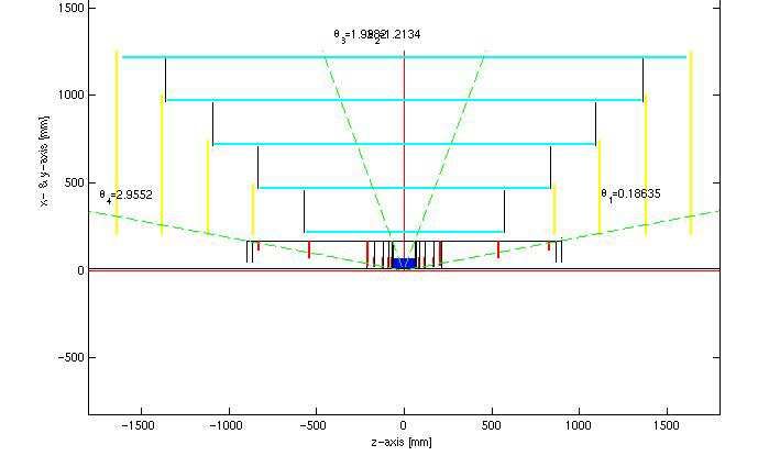
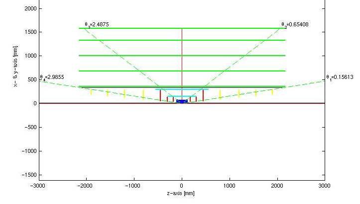
The algorithms used in the tool are on a solid mathematical basis. The software is written
in MatLab, a high-level matrix algebra language and IDE [3]. The tool is deliberately kept
simple and can without effort be adapted to meet individual needs. Its main purpose, however,
is to supply a tool for non-experts, without any knowledge of algorithmic details. Once the
detector description (“input sheet”) has been set up, individual detector layers can easily be
moved, removed or modified, and the result of these changes can quickly be evaluated. For ease
of use, the program is integrated into a graphical user interface (GUI), Figure 1.

Figure 1a: “LiC Detector Toy” GUI – the main menu.

The tool was beta released at the VCI 2007 [4]. For a
thorough description of its functionality and usage see
refs. [4, 5].                                                   Figure 1b: setting parameters.

2. Track resolution study
This study is based on about 2 × 18, 700 (LDC barrel), 22,400 (SiD barrel) and 8,840
(LDC forward/backward) tracks, respectively, simulated and fitted by the “LiC Detector Toy”
program. Definitions of the “barrel” and “forward/backward” regions in terms of the dip angle
λ ≡ π/2 − ϑpolar are given in section 3.
   The true and fitted track data are passed to and further analyzed by a Java program, running
within JAS3 and using AIDA [6]: calculating the deviations of fitted w.r.t. true transverse
momenta ∆pT = (pfTitted − pT ), and the impact parameters δT and δ0 (transverse and in space,
respectively); histogramming ∆pT /pT , ∆pT /p2T , δT and δ0 for separate intervals of true pT ;
extracting the rms or mean from each histogram; then using parametrizations (subsection 2.2)
to fit rms(∆pT /pT ), rms(∆pT /p2T ), rms(δT ), and mean(δ0 ) as functions of the central value of
each pT interval – see Figures 3 . . . 6.
   Section 3 presents preliminary results, and section 4 the conclusions.

2.1. LDC and SiD detector descriptions
The geometry and material constants of the ILC “Large Detector” (LDC) and “Silicon Detector”
(SiD) concepts have been taken from their 2006 Detector Outline Documents [7]; recent updates
are taken into account. Visualization snapshots of the layouts and summaries of the detector
descriptions are shown in Figure 2.
The LDC concept:                                                                                    The SiD concept:

                               LDC Detector description
                                                                                                                                    SiD Detector description
                  Bz = 4 Tesla; efficiency Si = 95%, TPC = 100%; errors in m
                                                                                                                             Bz = 5 Tesla; efficiency Si = 95%; errors in m
  BARREL           R[mm]   Zmin[mm]       Zmax[mm]    Error distribution   d[Xo]         Remarks
  Beam pipe             14                            passive                      .0025 0.4 mm         BARREL         R[mm]    Zmin[mm] Zmax[mm]      Error distribution      d[Xo]       Remarks
                                                                                         Be             Beam pipe            12       -62.5       62.5 passive                      .00253 0.4 mm
  VTX 1                 16         -50           50 pads 50*50 (25*25)              .002 wafer +                                   + conus     + conus                                     Be + Ti
                                                    equ. distrib.                        ladder         VXD 1              14.6       -62.5       62.5 pads 20*20                   .00202 wafer +
  VTX 2                 26      -120            120 idem                   idem          idem                                                          equ. distrib.                       ladder
  VTX 3                 37 idem      idem           idem                   idem          idem           VXD 2              22.6 idem        idem       idem                    idem        idem
  VTX 4                 48 idem      idem           idem                   idem          idem           VXD 3              35.4 idem        idem       idem                    idem        idem
  VTX 5                 60 idem      idem           idem                   idem          idem           VXD 4              48.0 idem        idem       idem                    idem        idem
  Support               90      -110            -90 passive                         .070 arbitrary      VXD 5              60.4 idem        idem       idem                    idem        idem
  structures                                                                                            Dbl. support      168.7      -868.8      868.8 passive                         2 * dbl. wall
  idem                idem         90       110 passive                    idem        idem             cylinders         184.2      -894.3      894.3                              .00152 C fibre
  SIT 1                150       -150       150 strips 2*50                      .0175 0 o, 10o         TRK 1             218.0      -558.0      558.0 strips 50                    .00800 single
  SIT 2                290       -360       360 idem                       idem        idem             TRK 2             468.0      -825.0      825.0 idem                    idem        idem
  TPC inn. wall        340      -2160      2160 passive                          0.140                  TRK 3             718.0    -1083.0      1083.0 idem                    idem        idem
  196 pad rings       2.5 GeV as:
    σ(δT,0 ) = a + b · e−pT /c     (for high pT , the asymptotic value = a)
  • In the forward/backward region, only linear parametrizations in pT > 2.5 GeV have been
    used; thus the divergent part of σ(pT )/p2T is cut away.

2.3. LDC and SiD track resolutions
  • LDC and SiD barrel regions for pT = 2.5 . . . 35 GeV (Figures 3 . . . 6 at left):
    the data points correspond to LDC 50 × 50µm pixels (blue dots), LDC 25 × 25µm pixels
    (red squares), and SiD 20 × 20µm pixels (purple triangles), respectively, of the barrel vertex
    detectors - for a detailed description, see subsection 2.1.
  • LDC forward/backward regions for pT = 2.5 . . . 25 GeV (Figures 3 . . . 6 at right):
    the data points correspond to dip angle ranges of 81o < |λ| < 81.5o (blue dots),
    81.5o < |λ| < 82o (red squares), and 82o < |λ| < 82.5o (purple triangles).
The values are averages over pT intervals of width 2.5 GeV. The error bars shown reflect only the statistics normalized to bin content. Figure 3: rms(∆pT /pT ) vs. pT for barrel (left) and forward/backward (right) regions. Figure 4: rms(∆pT /p2T ) [GeV−1 ] vs. pT for barrel (left) and forward/backward (right) regions. Figure 5: rms(δT ) [mm] vs. pT for barrel (left) and forward/backward (right) regions. Figure 6: mean(δ0 ) [mm] vs. pT for barrel (left) and forward/backward (right) regions.
3. Preliminary results
The results extracted from Figures 3 . . . 6 (subsection 2.3) are summarized below.
Barrel regions (LDC: |λ| < 48o , SiD: |λ| < 20o ), pT = 2.5 . . . 35 GeV:
      Detector, px size      rms(∆pT /pT )              rms(∆pT /p2T ) [GeV−1 ]     rms(δT )2    mean(δ0 )2

      LDC 50 × 50µm          (4.6 · pT + 30.7) · 10−5   (4.5 + 31.9/pT ) · 10−5     7.69 µm      9.56 µm
      LDC 25 × 25µm          (4.6 · pT + 28.5) · 10−5   (4.6 + 29.5/pT ) · 10−5     4.29 µm      5.91 µm
      SiD 20 × 20µm          (2.4 · pT + 140.) · 10−5   (2.2 + 144./pT ) · 10−5     3.46 µm      6.46 µm

Forward/backward regions (81o < |λ| < 82.5o ), pT = 2.5 . . . 25 GeV:
      LDC |λ| range          rms(∆pT /pT )              rms(∆pT /p2T )3              rms(δT )2   mean(δ0 )2

      81o < |λ| < 81.5o      (8.4 · pT − 2.83) · 10−3   8.36 · 10−3 GeV−1            86.7 µm     70.7 µm
      81.5o < |λ| < 82o      (5.7 · pT + 0.35) · 10−3   5.80 · 10−3 GeV−1            70.3 µm     57.1 µm
      82o < |λ| < 82.5o      (5.0 · pT + 3.65) · 10−3   5.37 · 10−3 GeV−1            63.1 µm     53.4 µm

4. Conclusions
In the barrel region and for transverse momenta pT < 35 GeV, the momentum resolution benefits
dramatically from the low material budget of LDC’s TPC. In contrast, SiD’s all-Si tracker
suffers from repeated “breakpoints” due to multiple scattering which forbids fitting a sufficiently
long undisturbed track segment (as in a TPC); we have proved for pT = 5 . . . 7.5 GeV that
hypothetically reducing SiD’s material budget to a quarter would halve rms(∆pT /pT ). However,
extrapolation to higher momenta shows a break-even at pT ≈ 50 GeV, as expected.
   The transverse impact parameters in the barrel region reflect directly the resolutions (i.e. the
pixel sizes) of the corresponding vertex detector’s innermost layer(s).
   In the forward/backward region |λ| > 81o , the momentum resolution is sensitive to LDC’s
forward tracker strips stereo angle: ±45o (i.e. perpendicular orientation) is a good compromise
between optimal R − Φ and R − z resolutions. The transverse impact parameters and those in
space are almost identical; emphasis must rather be given to ∆z (not shown).
   For the extreme forward/backward region |λ| > 82.5o (not shown), track reconstruction
suffers extremely from inefficiencies, and might require non-standard treatment.

References
    [1] R. Frühwirth et al.: Data Analysis Techniques for High-Energy-Physics, 2nd edition (eds. M. Regler and
          R. Frühwirth), Cambridge University Press (2000).
    [2] M. Regler, R. Frühwirth and W. Mitaroff: Int.J.Mod.Phys. C7, 4 (1996) 521.
        R. Frühwirth et al.: Nucl.Instr. Meth. A 334 (1993) 528.
    [3] D. Hanselmann and B. Littlefield: Mastering MatLab 7 , Pearson Prentice-Hall (2005).
        See also http://www.mathworks.com/
    [4] M. Regler, M. Valentan and R. Frühwirth: The LiC Detector Toy Program, Proc. 11th Vienna Conf. on
          Instrumentation (VCI) 2007, Nucl.Instr.Meth. A (in print).
    [5] User’s Guide: http://wwwhephy.oeaw.ac.at/p3w/ilc/reports/LiC_Det_Toy/Reports/UserGuide.pdf
    [6] FreeHep software used:
          Java Analysis Studio (JAS3): http://jas.freehep.org/
          Abstract Interfaces for Data Analysis (AIDA): http://aida.freehep.org/
    [7] ILC Detector Outline Documents:
          LDC (July 2006): http://www.ilcldc.org/documents/dod/outline.pdf
          SiD (May 2006): http://hep.uchicago.edu/~oreglia/siddod.pdf

2
     asymptotic value,
3
     weighted average.
You can also read